Performance Tuning Guide
Overview
Intel® Extension for PyTorch* is a Python package to extend official PyTorch. It makes the out-of-box user experience of PyTorch CPU better while achieving good performance. To fully utilize the power of Intel® architecture and thus yield high performance, PyTorch, as well as Intel® Extension for PyTorch*, are powered by oneAPI Deep Neural Network Library (oneDNN), an open-source cross-platform performance library of basic building blocks for deep learning applications. It is developed and optimized for Intel Architecture Processors, Intel Processor Graphics, and Xe architecture-based Graphics.
Although default primitives of PyTorch and Intel® Extension for PyTorch* are highly optimized, there are things users can do improve performance. Most optimized configurations can be automatically set by the launcher script. This article introduces common methods recommended by Intel developers.
Contents of this Document
Hardware Configuration
This section briefly introduces the structure of Intel CPUs, as well as concept of Non-Uniform Memory Access (NUMA).
Intel CPU Structure
There are many families of Intel CPUs. We’ll use Intel® Xeon® processor Scalable family as an example to discuss an Intel CPU and how it works. Understanding this background knowledge is helpful to understand the PyTorch optimization methodologies that Intel engineers recommend.
On the Intel® Xeon® Scalable Processors with Intel® C620 Series Chipsets, (formerly Purley) platform, each chip provides up to 28 cores. Each core has a non-inclusive last-level cache and an 1MB L2 cache. The CPU features fast 2666 MHz DDR4 memory, six memory channels per CPU, Intel Ultra Path Interconnect (UPI) high speed point-to-point processor interconnect, and more. Figure 1 shows microarchitecture of the Intel® Xeon® processor Scalable family chips. Each CPU chip consists of a number of cores, along with core-specific cache. 6 channels of DDR4 memory are connected to the chip directly. Meanwhile, chips communicates through the Intel UPI interconnect, which features a transfer speed of up to 10.4 GT/s.
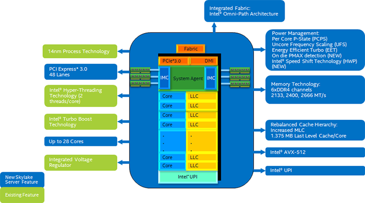
Figure 1: Block Diagram of the Intel® Xeon® processor Scalable family microarchitecture.
Usually, a CPU chip is called a socket. A typical two-socket configuration is illustrated as Figure 2. Two CPU sockets are equipped on one motherboard. Each socket is connected to up to 6 channels of memory, called its local memory, from socket perspective. Sockets are connected to each other via Intel UPI. It is possible for each socket to access memories attached on other sockets, usually called remote memory access. Local memory access is always faster than remote memory access. Meanwhile, cores on one socket share a space of high speed cache memory, which is much faster than communication via Intel UPI. Figure 3 shows an ASUS Z11PA-D8 Intel® Xeon® server motherboard, equipping with two sockets for Intel® Xeon® processor Scalable family CPUs.

Figure 2: Typical two-socket configuration.
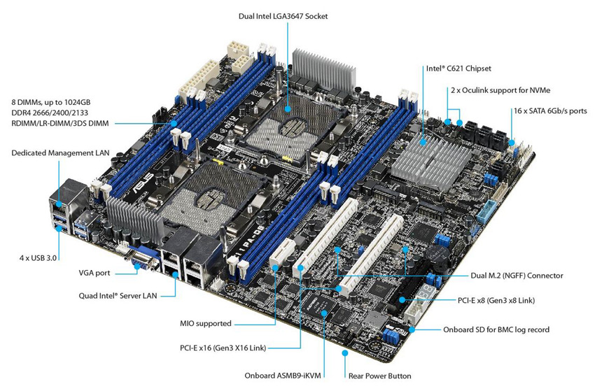
Figure 3: An ASUS Z11PA-D8 Intel® Xeon® server motherboard. It contains two sockets for Intel® Xeon® processor Scalable family CPUs.
Non-Uniform Memory Access (NUMA)
It is a good thing that more and more CPU cores are provided to users in one socket, because this brings more computation resources. However, this also brings memory access competitions. Program can stall because memory is busy to visit. To address this problem, Non-Uniform Memory Access (NUMA) was introduced. Comparing to Uniform Memory Access (UMA), in which scenario all memories are connected to all cores equally, NUMA tells memories into multiple groups. Certain number of memories are directly attached to one socket’s integrated memory controller to become local memory of this socket. As described in the previous section, local memory access is much faster than remote memory access.
Users can get CPU information with lscpu command on Linux to learn how many cores, sockets there on the machine. Also, NUMA information like how CPU cores are distributed can also be retrieved. The following is an example of lscpu execution on a machine with two Intel(R) Xeon(R) Platinum 8180M CPUs. 2 sockets were detected. Each socket has 28 physical cores onboard. Since Hyper-Threading is enabled, each core can run 2 threads. I.e. each socket has another 28 logical cores. Thus, there are 112 CPU cores on service. When indexing CPU cores, usually physical cores are indexed before logical core. In this case, the first 28 cores (0-27) are physical cores on the first NUMA socket (node), the second 28 cores (28-55) are physical cores on the second NUMA socket (node). Logical cores are indexed afterward. 56-83 are 28 logical cores on the first NUMA socket (node), 84-111 are the second 28 logical cores on the second NUMA socket (node). Typically, running Intel® Extension for PyTorch* should avoid using logical cores to get a good performance.
$ lscpu
...
CPU(s):              112
On-line CPU(s) list: 0-111
Thread(s) per core:  2
Core(s) per socket:  28
Socket(s):           2
NUMA node(s):        2
...
Model name:          Intel(R) Xeon(R) Platinum 8180M CPU @ 2.50GHz
...
NUMA node0 CPU(s):   0-27,56-83
NUMA node1 CPU(s):   28-55,84-111
...
Software Configuration
This section introduces software configurations that helps to boost performance.
Channels Last
Take advantage of Channels Last memory format for image processing tasks. Comparing to PyTorch default NCHW (torch.contiguous_format) memory format, NHWC (torch.channels_last) is more friendly to Intel platforms, and thus generally yields better performance. More detailed introduction can be found at Channels Last page. You can get sample codes with Resnet50 at Example page.
Numactl
Since NUMA largely influences memory access performance, this functionality should also be implemented in software side.
During development of Linux kernels, more and more sophisticated implementations/optimizations/strategies had been brought out. Version 2.5 of the Linux kernel already contained basic NUMA support, which was further improved in subsequent kernel releases. Version 3.8 of the Linux kernel brought a new NUMA foundation that allowed development of more efficient NUMA policies in later kernel releases. Version 3.13 of the Linux kernel brought numerous policies that aim at putting a process near its memory, together with the handling of cases such as having memory pages shared between processes, or the use of transparent huge pages. New sysctl settings allow NUMA balancing to be enabled or disabled, as well as the configuration of various NUMA memory balancing parameters.[1] Behavior of Linux kernels are thus different according to kernel version. Newer Linux kernels may contain further optimizations of NUMA strategies, and thus have better performances. For some workloads, NUMA strategy influences performance great.
Linux provides a tool, numactl, that allows user control of NUMA policy for processes or shared memory. It runs processes with a specific NUMA scheduling or memory placement policy. As described in previous section, cores share high-speed cache in one socket, thus it is a good idea to avoid cross socket computations. From a memory access perspective, bounding memory access locally is much faster than accessing remote memories.
The following is an example of numactl usage to run a workload on the Nth socket and limit memory access to its local memories on the Nth socket. More detailed description of numactl command can be found on the numactl man page.
numactl --cpunodebind N --membind N python <script>
Assume core 0-3 are on socket 0, the following command binds script execution on core 0-3, and binds memory access to socket 0 local memories.
numactl --membind 0 -C 0-3 python <script>
OpenMP
OpenMP is an implementation of multithreading, a method of parallelizing where a primary thread (a series of instructions executed consecutively) forks a specified number of sub-threads and the system divides a task among them. The threads then run concurrently, with the runtime environment allocating threads to different processors.[2] Figure 4 illustrates fork-join model of OpenMP execution.
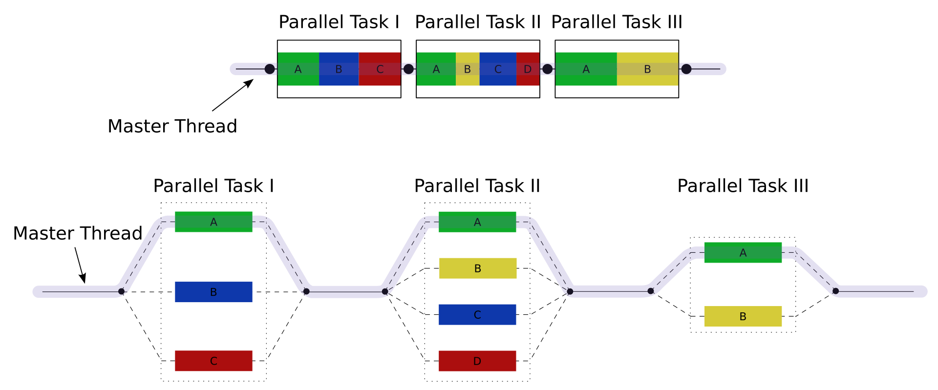
Figure 4: A number of parallel block execution threads are forked from primary thread.
Users can control OpenMP behaviors through some environment variables to fit for their workloads. Also, beside GNU OpenMP library (libgomp), Intel provides another OpenMP implementation libiomp for users to choose from. Environment variables that control behavior of OpenMP threads may differ from libgomp and libiomp. They will be introduced separately in sections below.
GNU OpenMP (libgomp) is the default multi-threading library for both PyTorch and Intel® Extension for PyTorch*.
OMP_NUM_THREADS
Environment variable OMP_NUM_THREADS sets the number of threads used for parallel regions. By default, it is set to be the number of available physical cores. It can be used along with numactl settings, as the following example. If cores 0-3 are on socket 0, this example command runs <script> on cores 0-3, with 4 OpenMP threads.
This environment variable works on both libgomp and libiomp.
export OMP_NUM_THREADS=4
numactl -C 0-3 --membind 0 python <script>
OMP_THREAD_LIMIT
Environment variable OMP_THREAD_LIMIT specifies the number of threads to use for the whole program. The value of this variable shall be a positive integer. If undefined, the number of threads is not limited.
Please make sure OMP_THREAD_LIMIT is set to a number equal to or larger than OMP_NUM_THREADS to avoid backward propagation hanging issues.
GNU OpenMP
Beside OMP_NUM_THREADS, other GNU OpenMP specific environment variables are commonly used to improve performance:
GOMP_CPU_AFFINITY: Binds threads to specific CPUs. The variable should contain a space-separated or comma-separated list of CPUs.OMP_PROC_BIND: Specifies whether threads may be moved between processors. Setting it to CLOSE keeps OpenMP threads close to the primary thread in contiguous place partitions.OMP_SCHEDULE: Determine how OpenMP threads are scheduled.
Here are recommended settings of these environment variables:
export GOMP_CPU_AFFINITY="0-3"
export OMP_PROC_BIND=CLOSE
export OMP_SCHEDULE=STATIC
Intel OpenMP
By default, PyTorch uses GNU OpenMP (GNU libgomp) for parallel computation. On Intel platforms, Intel OpenMP Runtime Library (libiomp) provides OpenMP API specification support. It sometimes brings more performance benefits compared to libgomp. Utilizing environment variable LD_PRELOAD can switch OpenMP library to libiomp:
pip install intel-openmp=2024.1.2
export LD_PRELOAD=<path>/libiomp5.so:$LD_PRELOAD
Similar to GNU OpenMP, beside OMP_NUM_THREADS, there are other Intel OpenMP specific environment variables that control behavior of OpenMP threads:
KMP_AFFINITYKMP_AFFINITYcontrols how to to bind OpenMP threads to physical processing units. Depending on the system (machine) topology, application, and operating system, thread affinity can have a dramatic effect on the application speed.A common usage scenario is to bind consecutive threads close together, as is done with KMP_AFFINITY=compact. By doing this, communication overhead, cache line invalidation overhead, and page thrashing are minimized. Now, suppose the application also had a number of parallel regions that did not utilize all of the available OpenMP threads. A thread normally executes faster on a core where it is not competing for resources with another active thread on the same core. It is always good to avoid binding multiple threads to the same core while leaving other cores unused. This can be achieved by the following command. Figure 5 illustrates this strategy.
export KMP_AFFINITY=granularity=fine,compact,1,0
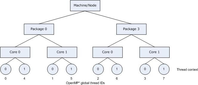
Figure 5: KMP_AFFINITY=granularity=fine,compact,1,0
The OpenMP thread n+1 is bound to a thread context as close as possible to OpenMP thread n, but on a different core. Once each core has been assigned one OpenMP thread, the subsequent OpenMP threads are assigned to the available cores in the same order, but they are assigned on different thread contexts.
It is also possible to bind OpenMP threads to certain CPU cores with the following command.
export KMP_AFFINITY=granularity=fine,proclist=[N-M],explicit
More detailed information about
KMP_AFFINITYcan be found in the Intel CPP Compiler Developer Guide.KMP_BLOCKTIMEKMP_BLOCKTIMEsets the time, in milliseconds, that a thread, after completing the execution of a parallel region, should wait before sleeping. The default value is 200ms.After completing the execution of a parallel region, threads wait for new parallel work to become available. After a certain period of time has elapsed, they stop waiting and sleep. Sleeping allows the threads to be used, until more parallel work becomes available, by non-OpenMP threaded code that may execute between parallel regions, or by other applications. A small
KMP_BLOCKTIMEvalue may offer better overall performance if application contains non-OpenMP threaded code that executes between parallel regions. A largerKMP_BLOCKTIMEvalue may be more appropriate if threads are to be reserved solely for use for OpenMP execution, but may penalize other concurrently-running OpenMP or threaded applications. It is suggested to be set to 0 or 1 for convolutional neural network (CNN) based models.export KMP_BLOCKTIME=0 (or 1)
Memory Allocator
Memory allocator plays an important role from performance perspective as well. A more efficient memory usage reduces overhead on unnecessary memory allocations or destructions, and thus results in a faster execution. From practical experiences, for deep learning workloads, Jemalloc or TCMalloc can get better performance by reusing memory as much as possible than default malloc function.
It is as simple as adding path of Jemalloc/TCMalloc dynamic library to environment variable LD_PRELOAD to switch memory allocator to one of them.
export LD_PRELOAD=<jemalloc.so/tcmalloc.so>:$LD_PRELOAD
Jemalloc
Jemalloc is a general purpose malloc implementation that emphasizes fragmentation avoidance and scalable concurrency support. More detailed introduction of performance tuning with Jemalloc can be found at Jemalloc tuning guide
A recommended setting for MALLOC_CONF is oversize_threshold:1,background_thread:true,metadata_thp:auto,dirty_decay_ms:9000000000,muzzy_decay_ms:9000000000 from performance perspective. However, in some cases the dirty_decay_ms:9000000000,mmuzzy_decay_ms:9000000000 may cause Out-of-Memory crash. Try oversize_threshold:1,background_thread:true,metadata_thp:auto instead in this case.
Getting Jemalloc is straight-forward.
conda install -c conda-forge jemalloc
TCMalloc
TCMalloc also features a couple of optimizations to speed up program executions. One of them is holding memory in caches to speed up access of commonly-used objects. Holding such caches even after deallocation also helps avoid costly system calls if such memory is later re-allocated. It is part of gpertools, a collection of a high-performance multi-threaded malloc() implementation, plus some pretty nifty performance analysis tools.
Getting TCMalloc is also not complicated.
conda install -c conda-forge gperftools
Denormal Number
Denormal number is used to store extremely small numbers that are close to 0. Computations with denormal numbers are remarkably slower than normalized number. To solve the low performance issue caused by denormal numbers, users can use the following PyTorch API function.
torch.set_flush_denormal(True)
OneDNN primitive cache
Intel® Extension for PyTorch* is using OneDNN backend for those most computing bound PyTorch operators such as Linear and Convolution.
To achieve better performance, OneDNN backend is using its primitive cache to store those created primitives for different input shapes during warm-up stage (default primitive cache size is 1024, i.e., 1024 cached primitives). Therefore, when the total size of the primitives created by all the input shapes is within the default threshold, Intel® Extension for PyTorch* could get fully computation performance from OneDNN kernels.
Different input shapes usualy come from dynamic shapes of datasets. Dynamic shapes commonly exist in MaskRCNN model (object detection), Transformers Wav2vec2 model (speech-recognition) and other speech/text-generation related Transformers models.
However, we might meet the fact that model would need to cache a large amount of various input shapes, which would even exceed the default primitive cache size. In such case, we recommend tuning the OneDNN primitive cache by setting ONEDNN_PRIMITIVE_CACHE_CAPACITY environment variable to get better performance (Note that it is at the cost of increased memory usage):
export ONEDNN_PRIMITIVE_CACHE_CAPACITY = {Tuning size}
//Note that {Tuning size} has an upper limit 65536 cached primitives
Take Transformers Wav2vec2 for speech-recognition as an example, the dataset “common voice” used for inference has a large amount of difference shapes for Convolution operator. In our experiment, the best primitive cache size is 4096, and the model runs with its full speed after being warmed up with inputs of all the shape sizes.