A Tour of GHZ examples

This tutorial provides some basic introduction to programming quantum algorithms and working with the FullStateSimulator through three implementations of the following circuit

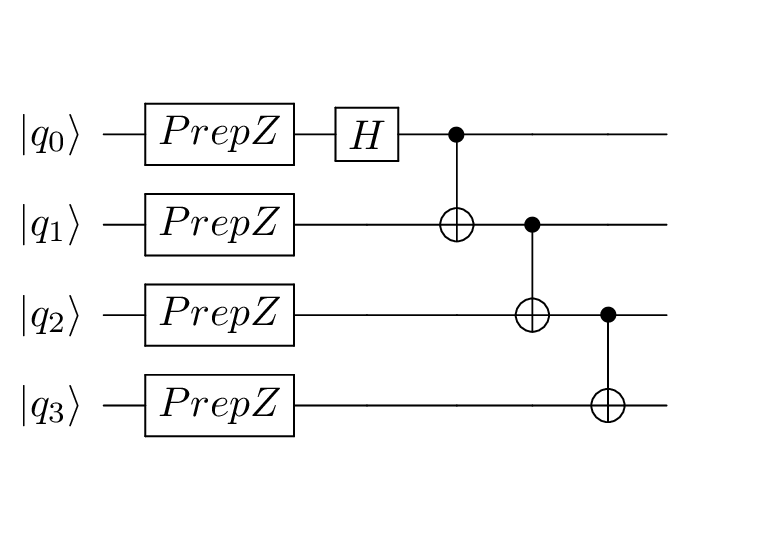
and the accompanying classical logic. The executable will manage running the above quantum circuit and retrieving the data in the FullStateSimulator to confirm the instructions are producing what is intended. This circuit produces a Greenberger-Horne-Zeilinger (GHZ) state for 4 qubits. In other words, the qubits will be in a super-position of two states, one with all qubits in the \(\ket{0}\) state and one with all qubits in the \(\ket{1}\) state, and each with equal chance of being measured.

The source code for each implementation is available in the quantum_examples/ directory of the Intel® Quantum SDK.

Ideal GHZ

To begin writing the program, get access to the quantum data types and methods by including the quintrinsics.h and the quantum_full_state_simulator_backend.h headers into the source as shown in Listing 2.

Listing 2 The headers required to use the quantum gates or FullStateSimulator.

#include <clang/Quantum/quintrinsics.h>

/// Quantum Runtime Library APIs
#include <quantum_full_state_simulator_backend.h>

As described in Writing New Algorithms, next declare an array of qubits (qbit) in the global namespace as show in Listing 3

Listing 3 Declaration of the qbit type variables in global namespace.

const int total_qubits = 4;
qbit qubit_register[total_qubits];

Next, implement the quantum algorithm by writing the functions or classes that contain the quantum logic. The quantum_kernel keyword should be in front of each function that builds the quantum algorithm. Shown in Listing 4, all the quantum instructions are placed in a single quantum_kernel. The first instruction is to initialize the state of each qubit by utilizing a for loop to call PrepZ() on the elements of the qbit array. Next, apply a Hadamard gate (H()) on the first qubit to set it into a superposition. And lastly, apply Controlled Not gates (CNOT()) on pairs of qubits to create entanglement between them.

Listing 4 quantum_kernel to prepare a Greenberger-Horne-Zeilinger state.

quantum_kernel void ghz_total_qubits() {
  for (int i = 0; i < total_qubits; i++) {
    PrepZ(qubit_register[i]);
  }

  H(qubit_register[0]);

  for (int i = 0; i < total_qubits - 1; i++) {
    CNOT(qubit_register[i], qubit_register[i + 1]);
  }
}

In the main function of the program, instantiate a FullStateSimulator object and use its ready() method, as shown in Listing 5. Do that as described in Configuring the FullStateSimulator, by first creating an IqsConfig object, changing it to be verbose (not required), and then using it as an argument to the FullStateSimulator constructor. Then use the return of the ready() method to trigger an early exit if something is wrong.

Listing 5 Setup of the FullStateSimulator. See Configuring the FullStateSimulator for a more detailed explanation.

int main() {
  iqsdk::IqsConfig settings(total_qubits, "noiseless");
  settings.verbose = true;
  iqsdk::FullStateSimulator quantum_8086(settings);
  if (iqsdk::QRT_ERROR_SUCCESS != quantum_8086.ready())
    return 1;

Next, prepare the classical data structures for working with simulation data. Create a set of id values to refer to the qubits of interest as shown in Listing 6. This is important because qbit variables do not necessarily specify a constant physical qubit in hardware; this mapping can be created and changed at various stages during program execution according to the compiler optimizations.

Listing 6 Declare and fill a std::vector with references to the elements of the qbit array.

  // get references to qbits
  std::vector<std::reference_wrapper<qbit>> qids;
  for (int id = 0; id < total_qubits; ++id) {
    qids.push_back(std::ref(qubit_register[id]));
  }

Now that the backend simulator is ready, call the quantum_kernel.

Listing 7 Call the quantum_kernel.

  ghz_total_qubits();

After this line during execution, the FullStateSimulator contains the state-vector data describing the qubits. Although there are facilities to conveniently specify every possible state for a set of qubits, this could be an overwhelming amount of data. Where possible, use the available constructors described in API Reference to configure a QssIndex object to refer to only the states of interest and store them in a vector. In Listing 8, two explicit strings formatted for 4 qubits are used to specify the two states.

Listing 8 Specifying the states of interest; this will be an argument used to collect data from the simulation.

  // use string constructor of Quantum State Space index to choose which
  // basis states' data is retrieved
  iqsdk::QssIndex state_a("|0000>");
  iqsdk::QssIndex state_b("|1111>");
  std::vector<iqsdk::QssIndex> bases;
  bases.push_back(state_a);
  bases.push_back(state_b);

Now access the probabilities for these two states through FullStateSimulator’s getProbabilities() method. Remember that ideally the GHZ state would only be in \(\ket{0000}\) or \(\ket{1111}\). So for this simulated circuit, when summing the probabilities of measuring in either \(\ket{0000}\) or \(\ket{1111}\), the sum should be 1.0.

Listing 9 The classical logic that checks a property of the state in the qubit register. This gets quantum results from simulation data at runtime.

  iqsdk::QssMap<double> probability_map;
  probability_map = quantum_8086.getProbabilities(qids, bases);

  double total_probability = 0.0;
  for (auto const & key_value : probability_map) {
    total_probability += key_value.second;
  }
  std::cout << "Sum of probability to measure fully entangled state: "
            << total_probability << std::endl;

Alternatively, display a formatted summary of the states to the console output with displayProbabilities() or displayAmplitudes().

Listing 10 Generate a quick, formatted display of the probabilities for the two states of interest printed to the console.

  quantum_8086.displayProbabilities(probability_map);

This program can be compiled with the default options. Configuring the qubit simulation in the Intel® Quantum Simulator creates a set of qubits with no limitation on their connectivity, in other words two-qubit operations (gates) can be applied between any pair of qubits.

$  <path to Intel Quantum SDK>/intel-quantum-compiler ideal_GHZ.cpp

Running the executable produces a line describing each quantum instruction because the verbose option was set to true when configuring the FullStateSimulator. That is followed by the line showing that total_probability is equal to 1 and the summary produced by displayProbabilities().

$ ./ideal_GHZ

- Run noiseless simulation (verbose mode)
Instruction #4 : ROTXY(phi = 1.5707, gamma = 1.57075)  on phys Q 0
Instruction #5 : ROTXY(phi = 0, gamma = 3.14154)  on phys Q 0
Instruction #6 : ROTXY(phi = 4.71229, gamma = 1.57075)  on phys Q 1
Instruction #7 : CPHASE(gamma = 3.1415) on phys Q0 and phys Q1
Instruction #8 : ROTXY(phi = 1.5707, gamma = 1.57075)  on phys Q 1
Instruction #9 : ROTXY(phi = 4.71229, gamma = 1.57075)  on phys Q 2
Instruction #10 : CPHASE(gamma = 3.1415) on phys Q1 and phys Q2
Instruction #11 : ROTXY(phi = 1.5707, gamma = 1.57075)  on phys Q 2
Instruction #12 : ROTXY(phi = 4.71229, gamma = 1.57075)  on phys Q 3
Instruction #13 : CPHASE(gamma = 3.1415) on phys Q2 and phys Q3
Instruction #14 : ROTXY(phi = 1.5707, gamma = 1.57075)  on phys Q 3
Sum of probability to measure fully entangled state: 1
Printing probability map of size 2
|0000>  : 0.5                           |1111>  : 0.5

The complete code is available as ideal_GHZ.cpp in the quantum_examples/ directory of the Intel® Quantum SDK.

Sampled GHZ

As discussed in Measurements using Simulated Quantum Backends, the state-vector probabilities that the above program uses are not data that quantum hardware is capable of returning. Consider the hypothetical scenario in which you now need to know how many times the quantum circuit must be run and evaluated in order to find the probability with the desired numerical accuracy. This can be done efficiently by using the simulation data.

Only the non-quantum_kernel sections of the ideal_GHZ.cpp program need changed to accomplish this. This can be done by using a different FullStateSimulator method after calling the quantum_kernel, as shown in Listing 11

Listing 11 code_samples/sample_GHZ.cpp

  // use sampling technique to simulate the results of many runs
  std::vector<std::vector<bool>> measurement_samples;
  unsigned total_samples = 1000;
  measurement_samples = quantum_8086.getSamples(total_samples, qids);

Each std::vector<bool> represents the observation of a state, each individual value represents the outcome of that qubit as arranged in the qids vector. The FullStateSimulator has a helper method to conveniently calculate the number of times a given state appears in an ensemble of observations.

Listing 12 code_samples/sample_GHZ.cpp

  // build a distribution of states
  iqsdk::QssMap<unsigned int> distribution =
          iqsdk::FullStateSimulator::samplesToHistogram(measurement_samples);

From this QssMap, calculate the estimate of the probability of observing each state.

Listing 13 The classical logic inspecting the results of sampling many simulated measurements.

  // print out the results
  std::cout << "Using " << total_samples
            << " samples, the distribution of states is:" << std::endl;
  for (const auto & entry : distribution) {
    double weight = entry.second;
    weight = weight / total_samples;

    std::cout << entry.first << " : " << weight << std::endl;
  }

This program can be compiled with the same command as the previous program.

$ <path to Intel Quantum SDK>/intel-quantum-compiler sample_GHZ.cpp

In addition to the same output from ideal_GHZ.cpp, the result of the samplesToHistogram() method is also printed out:

Using 1000 samples, the distribution of states is:
|0000> : 0.496
|1111> : 0.504

Because the IqsConfig used the default setting of a random seed (by not specifying one), this simulation will produce a different sequence of samples on subsequent executions and thus a slightly different estimate of the probability of observing each state.

The complete code is available as sample_GHZ.cpp in the quantum_examples/ directory of the Intel® Quantum SDK.

GHZ state on Quantum Dot Simulator

It takes the change of only a few lines of code to target another backend, as you can see by comparing sample_GHZ.cpp and qd_GHZ.cpp (e.g. using the diff CLI tool). As described in Quantum Dot Simulator Backend, the Quantum Dot Simulator (QD_Sim) adds to the state vector simulation by including details from the control signals that interact with quantum dot qubits. This creates additional computational overhead compared to the Intel® Quantum Simulator. The first change in this program is to reduce the size of the circuit to just a pair of qubits so the execution stays around a few seconds.

QD_Sim treats running sequential quantum_kernels and measurement gates differently than the Intel® Quantum Simulator (see Important Points on Quantum Dot Simulator). Although some programs could require alteration of their logic, the above program’s quantum_kernel and simulator usage is compatible with either backend. To change the qubit simulator, instead of the IqsConfig object switch to a DeviceConfig constructed with the argument "QD_SIM" as shown in Listing 14 (note the all capitals for the argument string).

Listing 14 Configuring the FullStateSimulator to use the Quantum Dot Simulator backend.

int main() {
  iqsdk::DeviceConfig qd_config("QD_SIM");
  iqsdk::FullStateSimulator quantum_8086(qd_config);

With this change of backend qubit simulation, the program must now be compiled with non-default options. The file intel-quantum-sdk-QDSIM.json points to a file describing a 6-qubit linear array. Use the -c flag to give the file’s location to the compiler, and specify placement and scheduling options with -p and -S.

$ <path to Intel Quantum SDK>/intel-quantum-compiler -c <path to Intel Quantum SDK>/intel-quantum-sdk-QDSIM.json -p trivial -S greedy qd_GHZ.cpp

QD_Sim produces its own output in addition to the output explicitly designed into the behavior of the program.

$ ./qd_GHZ.cpp

1688766838 time dependent evolution start time
sweep progress: calculation point=0 0%
sweep progress: calculation point=18199 10%
sweep progress: calculation point=36398 20%
sweep progress: calculation point=54597 30%
sweep progress: calculation point=72796 40%
sweep progress: calculation point=90994 50%
sweep progress: calculation point=109193 60%
sweep progress: calculation point=127392 70%
sweep progress: calculation point=145591 80%
sweep progress: calculation point=163790 90%
Time evolution took 2.568378 seconds
Fri Jul  7 14:54:01 2023
1688766841 time dependent evolution end time
Sum of probability to measure fully entangled state: 0.999983
Printing probability map of size 2
|00>    : 0.4998                        |11>    : 0.5002

Using 1000 samples, the distribution of states is:
|00> : 0.519
|11> : 0.481

The output starts with the backend’s simulation progress, followed by the familiar output in the program’s implementation. The probabilities reported by the FullStateSimulator are slightly different from the exact \(0.50\) because the Quantum Dot Simulator includes the simulation of the electronics controlling the quantum dots.

The complete code is available as qd_GHZ.cpp in the quantum_examples/ directory of the Intel® Quantum SDK.

Using release_quantum_state()

Using release_quantum_state() to indicate the intention to effectively abandon operating on the qubits can lead to greater reduction of the total operations when combined with -O1 optimization. Inconsequential operations can be removed, and in some cases this can include a measurement operation. Consider the following sample code. The first three quantum_kernel blocks build up the preparation and measurement of a state with three angles as input parameters.

#include <clang/Quantum/quintrinsics.h>
#include <quantum_full_state_simulator_backend.h>

qbit q[2];

quantum_kernel void PrepAll() {
  PrepZ(q[0]);
  PrepZ(q[1]);
}

//nothing special about this ansatz
quantum_kernel void Ansatz_Heisenberg (double angle0, double angle1, double angle2) {
  RX(q[0], angle0);
  RY(q[1], angle1);
  S(q[1]);
  CNOT(q[0], q[1]);
  RZ(q[1], angle2);
  CNOT(q[0], q[1]);
  Sdag(q[1]);
}

quantum_kernel double Measure_Heisenberg(){
  cbit c[3];

  CNOT(q[0], q[1]);
  MeasX(q[0], c[0]); // XX term
  MeasZ(q[1], c[1]); // ZZ term
  CZ(q[0], q[1]);
  MeasX(q[0], c[2]); //-YY term
  CZ(q[0], q[1]);
  CNOT(q[0], q[1]);

  release_quantum_state();

  return (1. -2. * (double) c[0]) + (1. -2. * (double) c[1]) + (1. + 2. * (double) c[2]);

}

The next quantum_kernel function calls the prior three blocks. This fourth function contains the release_quantum_state() call from above. The main() function calls VQE_Heisenberg() after setting up a FullStateSimulator.

quantum_kernel double VQE_Heisenberg(double angle0, double angle1, double angle2) {
  PrepAll();
  Ansatz_Heisenberg (angle0, angle1, angle2);

  return Measure_Heisenberg();  //note this QK will inherit the release for this function
}

int main(){
  iqsdk::IqsConfig settings(2, "noiseless");
  iqsdk::FullStateSimulator quantum_8086(settings);
  if (iqsdk::QRT_ERROR_SUCCESS != quantum_8086.ready())
    return 1;

  double debug1 = 1.570796;
  double debug2 = debug1 / 2;
  double debug3 = debug2 / 2;
  VQE_Heisenberg(debug1, debug2, debug3);
}

If this is compiled with -O0 flag and no optimization is performed, we expect each of the 3 measurement operations (MeasX, MeasZ, MeasX) to be called. Looking at the resulting .qs file confirms this:

	.globl	"_Z45VQE_Heisenberg(double, double, double).QBB.3.v.stub" // -- Begin function _Z45VQE_Heisenberg(double, double, double).QBB.3.v.stub
	.type	"_Z45VQE_Heisenberg(double, double, double).QBB.3.v.stub",@function
"_Z45VQE_Heisenberg(double, double, double).QBB.3.v.stub": // @"_Z45VQE_Heisenberg(double, double, double).QBB.3.v.stub"
// %bb.0:                               // %aqcc.quantum
	quprep QUBIT[0] (slice_idx=1)
	quprep QUBIT[1] (slice_idx=0)
	qurotxy QUBIT[0], @shared_variable_array[4], @shared_variable_array[0] (slice_idx=0)
	qurotxy QUBIT[1], @shared_variable_array[5], @shared_variable_array[1] (slice_idx=0)
	qurotz QUBIT[1], 1.570796e+00 (slice_idx=0)
	qurotxy QUBIT[1], 1.570796e+00, 4.712389e+00 (slice_idx=0)
	qucphase QUBIT[0], QUBIT[1], 3.141593e+00 (slice_idx=0)
	qurotxy QUBIT[1], 1.570796e+00, 1.570796e+00 (slice_idx=0)
	qurotz QUBIT[1], @shared_variable_array[6] (slice_idx=0)
	qurotxy QUBIT[1], 1.570796e+00, 4.712389e+00 (slice_idx=0)
	qucphase QUBIT[0], QUBIT[1], 3.141593e+00 (slice_idx=0)
	qurotxy QUBIT[1], 1.570796e+00, 1.570796e+00 (slice_idx=0)
	qurotz QUBIT[1], 4.712389e+00 (slice_idx=0)
	qurotxy QUBIT[1], 1.570796e+00, 4.712389e+00 (slice_idx=0)
	qucphase QUBIT[0], QUBIT[1], 3.141593e+00 (slice_idx=0)
	qurotxy QUBIT[1], 1.570796e+00, 1.570796e+00 (slice_idx=0)
	qurotxy QUBIT[0], 1.570796e+00, 4.712389e+00 (slice_idx=0)
	qumeasz QUBIT[0] @shared_cbit_array[0] (slice_idx=0)
	qurotxy QUBIT[0], 1.570796e+00, 1.570796e+00 (slice_idx=0)
	qumeasz QUBIT[1] @shared_cbit_array[1] (slice_idx=0)
	qucphase QUBIT[0], QUBIT[1], 3.141593e+00 (slice_idx=0)
	qurotxy QUBIT[0], 1.570796e+00, 4.712389e+00 (slice_idx=0)
	qumeasz QUBIT[0] @shared_cbit_array[2] (slice_idx=0)
	qurotxy QUBIT[0], 1.570796e+00, 1.570796e+00 (slice_idx=0)
	qucphase QUBIT[0], QUBIT[1], 3.141593e+00 (slice_idx=0)
	qurotxy QUBIT[1], 1.570796e+00, 4.712389e+00 (slice_idx=0)
	qucphase QUBIT[0], QUBIT[1], 3.141593e+00 (slice_idx=0)
	qurotxy QUBIT[1], 1.570796e+00, 1.570796e+00 (slice_idx=2)
	return
.Lfunc_end3:
	.size	"_Z45VQE_Heisenberg(double, double, double).QBB.3.v.stub", .Lfunc_end3-"_Z45VQE_Heisenberg(double, double, double).QBB.3.v.stub"
                                        // -- End function
	.section	".note.GNU-stack","",@progbits

However, compiling with -O1 will cause the optimizer to remove operations. Here in addition to combining and removing gates, the optimizer will remove a measurement operation because its outcome can be deduced from the other two measurements’ outcomes. The cbit used to store the now-missing measurement outcome will have its value correctly set by the Quantum Runtime.

	.globl	"_Z45VQE_Heisenberg(double, double, double).QBB.3.v.stub" // -- Begin function _Z45VQE_Heisenberg(double, double, double).QBB.3.v.stub
	.type	"_Z45VQE_Heisenberg(double, double, double).QBB.3.v.stub",@function
"_Z45VQE_Heisenberg(double, double, double).QBB.3.v.stub": // @"_Z45VQE_Heisenberg(double, double, double).QBB.3.v.stub"
// %bb.0:                               // %aqcc.quantum
	quprep QUBIT[1] (slice_idx=1)
	quprep QUBIT[0] (slice_idx=0)
	qurotxy QUBIT[1], @shared_variable_array[4], @shared_variable_array[1] (slice_idx=0)
	qurotxy QUBIT[0], @shared_variable_array[5], @shared_variable_array[0] (slice_idx=0)
	qurotxy QUBIT[0], 1.570796e+00, 4.712389e+00 (slice_idx=0)
	qurotxy QUBIT[1], 1.570796e+00, 0.000000e+00 (slice_idx=0)
	qucphase QUBIT[0], QUBIT[1], 3.141593e+00 (slice_idx=0)
	qurotxy QUBIT[0], 1.570796e+00, 0.000000e+00 (slice_idx=0)
	qumeasz QUBIT[0] @shared_cbit_array[0] (slice_idx=0)
	qurotxy QUBIT[1], 1.570796e+00, 4.712389e+00 (slice_idx=0)
	qumeasz QUBIT[1] @shared_cbit_array[1] (slice_idx=2)
	return
.Lfunc_end3:
	.size	"_Z45VQE_Heisenberg(double, double, double).QBB.3.v.stub", .Lfunc_end3-"_Z45VQE_Heisenberg(double, double, double).QBB.3.v.stub"
                                        // -- End function
	.section	".note.GNU-stack","",@progbits

Writing Variational Algorithms

Introduction

Variational algorithms are considered to be one of the most promising applications to allow quantum advantage using near-term systems [CAB+21]. The Intel® Quantum SDK has many features that are geared for coding variational algorithms with a focus on performance. The Hybrid Quantum Classical Library (HQCL) [IntelLabs23] is a collection of tools that will help a user increase productivity when programming variational algorithms. This example combines these tools with dlib (a popular C++ library for solving optimization problems [DLI23] ), to applying the variational algorithm to the generation of thermofield double (TFD) states [PM20] [SPK+21]. Previous implementations [KWP+22] included the latter workload with a hard-coded version of the cost function expression, which was pre-calculated. Fig. 1 (reproduced from [KWP+22]) shows the full circuit that is used for the variational algorithm execution.

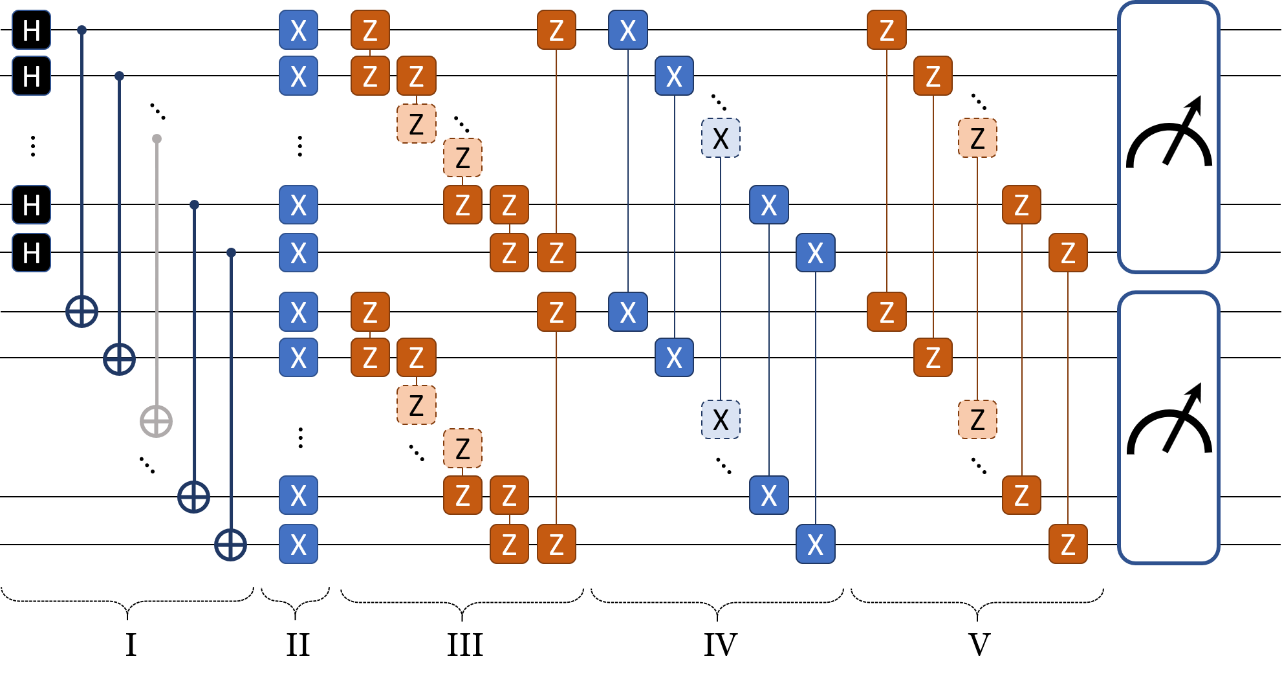
Fig. 1 The quantum circuit for single-step TFD state generation. Stages:(I) preparing infinite temperature TFD state, (II) Intra-system \(R_X\) operation, (III) Intra-system \(ZZ\) operation, (IV) Inter-system \(XX\) operation, (V) Inter-system \(ZZ\) operation. A and B represent the two subsystems, each containing \(N_\textrm{sub}\) qubits. (reproduced from [KWP+22])

In this implementation, HQCL will symbolically construct the cost function expression, and use qubit-wise commutation (QWC) [YVI20] to group terms and reduce the number of circuit repetitions required to calculate the cost function. HQCL will also automatically populate the necessary mapping angles at runtime, to facilitate measurements of the system along different axes.

The classical optimization in this workload will be handled using the dlib C++ library. The dlib library contains powerful functions performing local as well as global optimizations. Here, the find_min_bobyqa function for the minimization of the cost function performs quite well for the chosen workload. The choice of the optimization technique can heavily influence the number of iterations required for convergence of certain variational algorithms. The Intel Quantum Simulator [GHBS20] will be used as the backend in this example.

Code

Preamble

In the preamble of the source file shown in Listing 15 below, the header files for the IQSDK, dlib, and HQCL are included first.

Listing 15 The preamble of the source file.

// Intel Quantum SDK header files
#include <clang/Quantum/quintrinsics.h>
#include <quantum.hpp>

#include <vector>
#include <cassert>

// Library for optimizations
#include <dlib/optimization.h>
#include <dlib/global_optimization.h>

// Libraries for automating hybrid algorithm
#include <armadillo>
#include "SymbolicOperator.hpp"
#include "SymbolicOperatorUtils.hpp"

// Define the number of qubits needed for compilation
const int N_sub = 2;  // Number of qubits in subsystem (thermal state size)
const int N_ss = 2; // Number of subsystems (Not a general parameter to be changed)
const int N = N_ss * N_sub; // Total number of qubits (TFD state size)

qbit QReg[N];
cbit CReg[N];

const int N_var_angles = 4;
const int N_map_angles = 2 * N;

double QVarParams[N_var_angles]; // Array to hold dynamic parameters for quantum algorithm
double QMapParams[N_map_angles]; // Array to hold mapping parameters for HQCL

typedef dlib::matrix<double, N_var_angles, 1> column_vector;
namespace hqcl = hybrid::quantum::core;

A data structure within dlib is defined (using a typedef) in line 31 for convenience in passing the set of parameters into the optimization loop. This algorithm will use four variational parameters and two mapping angles per qubit (a total of eight).

Construction of the Ansatz

Listing 16 contains the operations corresponding to the stages II, III, IV, and V from Fig. 1 (stage I will be discussed later in Listing 17). These are the four core stages that define the operations for the TFD algorithm. A future version of the IQSDK will support quantum kernel expressions which can be used to conveniently construct quantum kernels in a modular way [PSM23] [Sch23].

Listing 16 The core set of operations to implement the TFD algorithm.

quantum_kernel void TFD_terms () {
  int index_intraX = 0, index_intraZ = 0, index_interX = 0, index_interZ = 0;

  // Single qubit variational terms
  for (index_intraX = 0; index_intraX < N; index_intraX++)
    RX(QReg[index_intraX], QVarParams[0]);

  // Two-qubit intra-system variational terms (adjacent)
  for (int grand_intraZ = 0; grand_intraZ < N_sub - 1; grand_intraZ++) {
    for (index_intraZ = 0; index_intraZ < N_ss; index_intraZ++)
      CNOT(QReg[grand_intraZ + N_sub * index_intraZ + 1], QReg[grand_intraZ + N_sub * index_intraZ]);
    for (index_intraZ = 0; index_intraZ < N_ss; index_intraZ++)
      RZ(QReg[grand_intraZ + N_sub * index_intraZ], QVarParams[1]);
    for (index_intraZ = 0; index_intraZ < N_ss; index_intraZ++)
      CNOT(QReg[grand_intraZ + N_sub * index_intraZ + 1], QReg[grand_intraZ + N_sub * index_intraZ]);
  }

  if (N_sub > 2) {
    // Two-qubit intra-system variational terms (boundary term)
    for (index_intraZ = 0; index_intraZ < N_ss; index_intraZ++)
      CNOT(QReg[N_sub * index_intraZ], QReg[N_sub * index_intraZ + (N_sub - 1)]);
    for (index_intraZ = 0; index_intraZ < N_ss; index_intraZ++)
      RZ(QReg[N_sub * index_intraZ + (N_sub - 1)], QVarParams[1]);
    for (index_intraZ = 0; index_intraZ < N_ss; index_intraZ++)
      CNOT(QReg[N_sub * index_intraZ], QReg[N_sub * index_intraZ + (N_sub - 1)]);
  }

  // two-qubit inter-system XX variational terms
  for (index_interX = 0; index_interX < N_sub; index_interX++) {
    RY(QReg[index_interX + N_sub], -M_PI_2);
    RY(QReg[index_interX], -M_PI_2);
  }
  for (index_interX = 0; index_interX < N_sub; index_interX++)
    CNOT(QReg[index_interX + N_sub], QReg[index_interX]);
  for (index_interX = 0; index_interX < N_sub; index_interX++)
    RZ(QReg[index_interX], QVarParams[2]);
  for (index_interX = 0; index_interX < N_sub; index_interX++)
    CNOT(QReg[index_interX + N_sub], QReg[index_interX]);
  for (index_interX = 0; index_interX < N_sub; index_interX++) {
    RY(QReg[index_interX + N_sub], M_PI_2);
    RY(QReg[index_interX], M_PI_2);
  }

  // two-qubit inter-system ZZ variational terms
  for (index_interZ = 0; index_interZ < N_sub; index_interZ++)
    CNOT(QReg[index_interZ], QReg[index_interZ + N_sub]);
  for (index_interZ = 0; index_interZ < N_sub; index_interZ++)
    RZ(QReg[index_interZ + N_sub], QVarParams[3]);
  for (index_interZ = 0; index_interZ < N_sub; index_interZ++)
    CNOT(QReg[index_interZ], QReg[index_interZ + N_sub]);

There are three supporting quantum kernels that are used (see Listing 17), in addition to the core set of operations. PrepZAll() is used to prepare all the qubits in the ground state at the beginning of every iteration. BellPrep() is used to prepare Bell pairs between corresponding qubits of the two subsystems, effectively resulting in the infinite temperature TFD state. The DynamicMapping() quantum kernel is used to hold the mapping operations that HQCL will implement for basis changes during runtime.

Listing 17 The supporting quantum kernels to implement the TFD algorithm.

quantum_kernel void PrepZAll () {
  // initialize the qubits
  for (int Index = 0; Index < N; Index++)
    PrepZ(QReg[Index]);
}

quantum_kernel void BellPrep () {
  // prepare the Bell pairs (T -> Infinity)
  for (int Index = 0; Index < N_sub; Index++)
    H(QReg[Index]);
  for (int Index = 0; Index < N_sub; Index++)
    CNOT(QReg[Index], QReg[Index + N_sub]);
}

quantum_kernel void DynamicMapping () {
  // Not part of the ansatz
  // Rotations to map X to Z or Y to Z
  for (int qubit_index = 0; qubit_index < N; qubit_index++) {
    int map_index = 2 * qubit_index;
    RY(QReg[qubit_index], QMapParams[map_index]);
    RX(QReg[qubit_index], QMapParams[map_index + 1]);
  }
}

The supporting quantum kernels (Listing 17) and the core TFD quantum kernel (Listing 16) are combined to form the full quantum circuit in Listing 18.

Listing 18 The full TFD quantum kernel to run during optimization loop.

quantum_kernel void TFD_full() {
  PrepZAll();
  BellPrep();
  TFD_terms();
  DynamicMapping();
}

Functions for Constructing the Cost Expression and the Cost Calculation

Listing 19 Construction of the full symbolic operator for the cost function expression.

hqcl::SymbolicOperator constructFullSymbOp(double inv_temp) {
  hqcl::SymbolicOperator symb_op;
  hqcl::pstring sym_term;

  // Single qubit variational terms
  for (int index_intraX = 0; index_intraX < N; index_intraX++) {
      sym_term = {std::make_pair(index_intraX, 'X')};
      symb_op.addTerm(sym_term, 1.00);
  }

  // Two-qubit intra-system variational terms (adjacent)
  for (int grand_intraZ = 0; grand_intraZ < N_sub - 1; grand_intraZ++) {
      for (int index_intraZ = 0; index_intraZ < N_ss; index_intraZ++) {
          int qIndex0 = grand_intraZ + N_sub * index_intraZ;
          int qIndex1 = grand_intraZ + N_sub * index_intraZ + 1;
          sym_term = {std::make_pair(qIndex0, 'Z'), std::make_pair(qIndex1, 'Z')};
          symb_op.addTerm(sym_term, 1.00);
      }
  }

  // Two-qubit intra-system variational terms (boundary term)
  if (N_sub > 2) {
      for (int index_intraZ = 0; index_intraZ < N_ss; index_intraZ++) {
          int qIndex0 = N_sub * index_intraZ;
          int qIndex1 = N_sub * index_intraZ + (N_sub - 1);
          sym_term = {std::make_pair(qIndex0, 'Z'), std::make_pair(qIndex1, 'Z')};
          symb_op.addTerm(sym_term, 1.00);
      }
  }

  // two-qubit inter-system XX variational terms
  for (int index_interX = 0; index_interX < N_sub; index_interX++) {
      int qIndex0 = index_interX;
      int qIndex1 = index_interX + N_sub;
      sym_term = {std::make_pair(qIndex0, 'X'), std::make_pair(qIndex1, 'X')};
      symb_op.addTerm(sym_term, -pow(inv_temp, -1.00));
  }

  // two-qubit inter-system XX variational terms
  for (int index_interZ = 0; index_interZ < N_sub; index_interZ++) {
      int qIndex0 = index_interZ;
      int qIndex1 = index_interZ + N_sub;
      sym_term = {std::make_pair(qIndex0, 'Z'), std::make_pair(qIndex1, 'Z')};
      symb_op.addTerm(sym_term, -pow(inv_temp, -1.00));
  }

  return symb_op;
}

Programmatic construction of the cost expression is necessary for HQCL to form the QWC groups, to generate the necessary circuits to run per optimization iteration, and to correctly evaluate the cost at each iteration. In Listing 19, we generate symbolic terms (sym_term) for every expression present, and add it to the full symbolic operator symb_op. The full cost expression to be coded is given by

\[\begin{split}C(\beta) &= \sum_{i=1}^{N_\textrm{sub}} {X_i^A} +\sum_{i=1}^{N_\textrm{sub}} {X_i^B} + \sum_{i=1}^{N_\textrm{sub}} {Z_i^A Z_{i+1}^A} + \sum_{i=1}^{N_\textrm{sub}} {Z_i^B Z_{i+1}^B} \\ &- \beta^{-1} \left( \sum_{i=1}^{N_\textrm{sub}} {X_i^A X_i^B} + \sum_{i=1}^{N_\textrm{sub}} {Z_i^A Z_i^B} \right)\end{split}\]

where the subscript represents the qubit index and the superscript represents the subsystem the qubit belongs to (A or B) [KWP+22].

Listing 20 A function to calculate the cost at each iteration during optimization.

double runQuantumKernel(iqsdk::FullStateSimulator &sim_device, const column_vector& params,
                   hqcl::SymbolicOperator &symb_op, hqcl::QWCMap &qwc_groups) {
  double total_cost = 0.0;

  for (auto &qwc_group : qwc_groups) {
    std::vector<double> variable_params;
    variable_params.reserve(N * 2);

    hqcl::SymbolicOperatorUtils::applyBasisChange(qwc_group.second, variable_params, N);

    std::vector<std::reference_wrapper<qbit>> qids;
    for (int qubit = 0; qubit < N; ++qubit)
      qids.push_back(std::ref(QReg[qubit]));

    // Set all the mapping angles to the default of 0.
    for (int map_index = 0; map_index < N_map_angles; map_index++)
      QMapParams[map_index] = 0;

    for (auto indx = 0; indx < variable_params.size(); ++indx)
      QMapParams[indx] = variable_params[indx];

    // Perform the experiment, Store the data in ProbReg
    TFD_full();
    std::vector<double> ProbReg = sim_device.getProbabilities(qids);

    double current_pstr_val = hqcl::SymbolicOperatorUtils::getExpectValSetOfPaulis(
        symb_op, qwc_group.second, ProbReg, N);
    total_cost += current_pstr_val;
  }

  return total_cost;
}

The function runQuantumKernel encompasses all the functionality that is required to calculate the cost, when running a single optimization iteration with dlib. It takes the already formulated set of QWC groups, and run the ansatz with the same set of variational parameters but with different basis mapping parameters (each time mapping from the different bases, as demanded by the cost expression). The full cost is then returned for consideration by the classical optimization loop within dlib.

Listing 21 The main function.

int main() {
    // Setup quantum device
    iqsdk::IqsConfig sim_config(N, "noiseless", false);
    iqsdk::FullStateSimulator sim_device(sim_config);
    assert(sim_device.ready() == iqsdk::QRT_ERROR_SUCCESS);

    // initial starting point. Defining it here means I will reuse the best result
    // from previous temperature when starting the next temperature run
    column_vector starting_point = {0, 0, 0, 0};

    // calculate the actual inverse temperature that is used during calculations
    double inv_temp = 1.0;

    // Fully formulated Cost Function Expression
    hqcl::SymbolicOperator cost_expr = constructFullSymbOp(inv_temp);

    // Qubitwise Commutation (QWC) Groups Formation
    hqcl::QWCMap qwc_groups = hqcl::SymbolicOperatorUtils::getQubitwiseCommutationGroups(cost_expr);

    // Construct a function to be used for a single optimization iteration
    // This function is directly called by the dlib optimization routine
    auto ansatz_run_lambda = [&](const column_vector& var_angs) {

      // Set all the variational angles to input values.
      for (int q_index = 0; q_index < N_map_angles; q_index++)
          QVarParams[q_index] = var_angs(q_index);

      // run the kernel to compute the total cost
      double total_cost = runQuantumKernel(sim_device, var_angs, cost_expr, qwc_groups);

      return total_cost;
    };

    // run the full optimization for a given temperature
    auto result = dlib::find_min_bobyqa(
                        ansatz_run_lambda, starting_point,
                        2 * N_var_angles + 1, // number of interpolation points
                        dlib::uniform_matrix<double>(N_var_angles, 1, -7.0), // lower bound constraint
                        dlib::uniform_matrix<double>(N_var_angles, 1, 7.0), // upper bound constraint
                        1.5, // initial trust region radius
                        1e-5, // stopping trust region radius
                        10000 // max number of objective function evaluations
    );

    return 0;
}

The main function shown in Listing 21 will initialize the IQSDK backend, construct the cost expression, and kick off the optimization. The lambda function ansatz_run_lambda is used since dlib requires the function used during optimization to take a column vector as an input and to return a double. This function essentially wraps the previously-defined runQuantumKernel function.

Results

The execution of the above program can be tracked with a log of the angles and the cost function at each iteration. The summarized results are shown in Fig. 2 and Fig. 3. These plots demonstrate that 95 steps are required for convergence to the requested tolerance level.

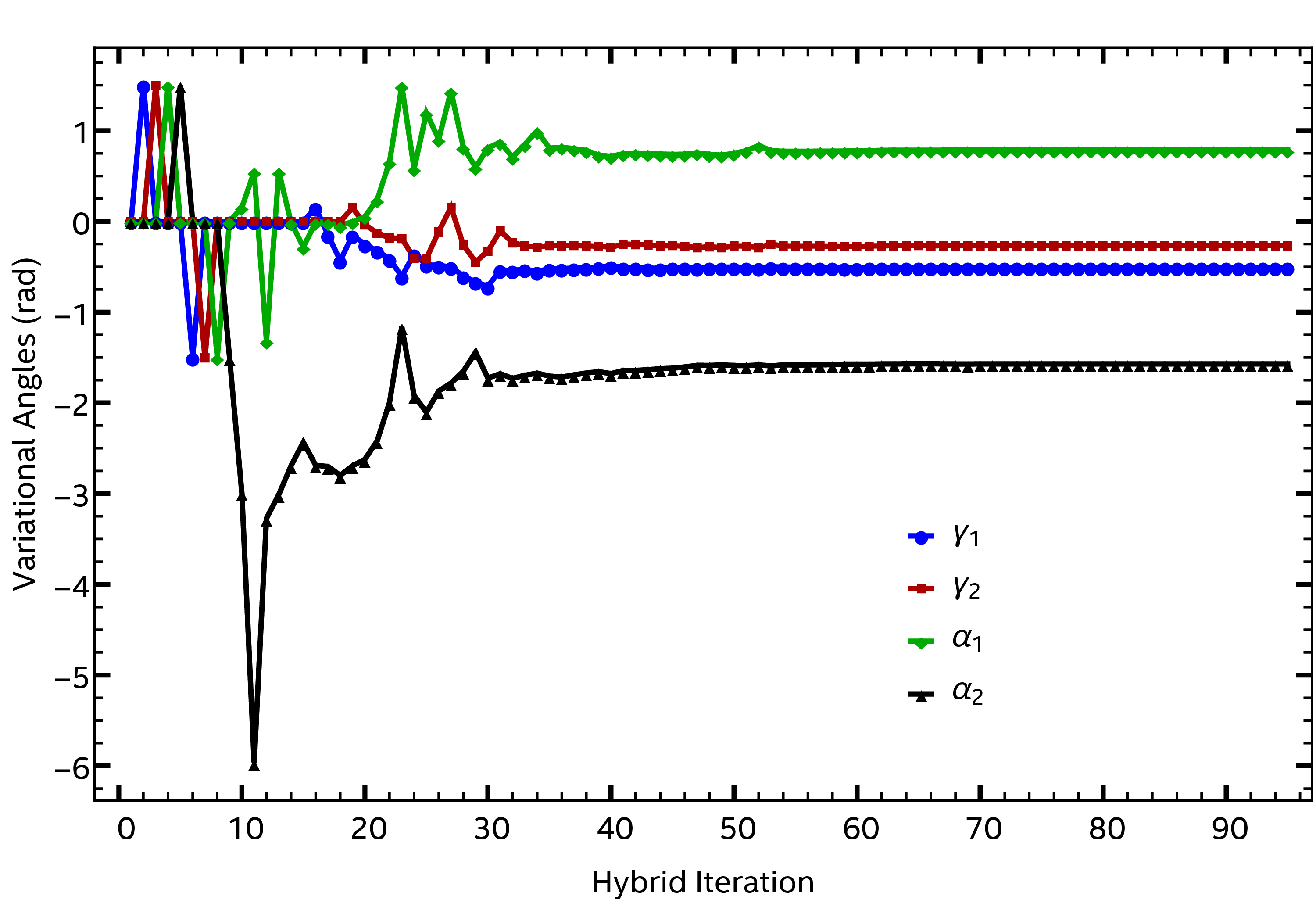
Fig. 2 Convergence behavior for the four variational angles (see [PM20] [SPK+21] for details on the notation).

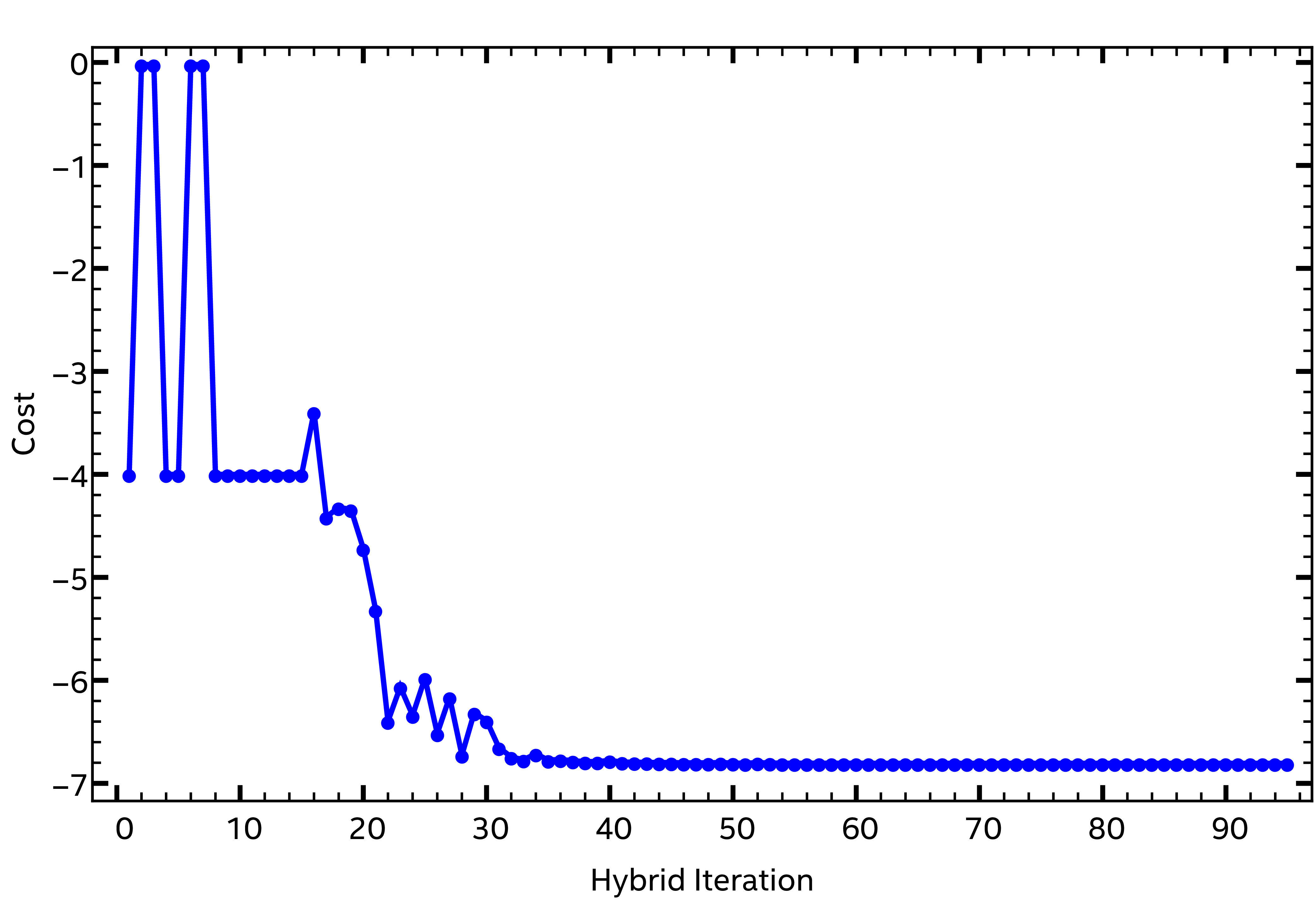
Fig. 3 Convergence of the evaluated cost during the variational algorithm execution.

Using qbit variables

qbit is the data type for representing qubits. Variables of qbit type can be declared in the global namespace or locally within a quantum_kernel function. Similar to locally declared classical C++ variables, locally declared qbit variables’ scope is limited to the quantum_kernel function they are declared in.

When a locally declared qbit variable goes out of scope, the quantum state is not automatically released. This means in subsequent computation, the physical qubit associated to this variable might be reassgined to a different qbit while still holding the now out-of-scope variable’s quantum state. Without proper handling, this could lead to unreliable results. One option is to use release_quantum_state() at the end of the quantum_kernel in which local qbit variables are declared. See Local qbit Variables. Examples can be found below:

qbit global_qbit;

void quantum_kernel exampleReleaseOnMeasurement(){
   qbit local_3[3];     // declare a quantum array with 3 qbits

   // Prep the local qbit variables
   PrepZ(local_3[0]);
   PrepZ(local_3[1]);
   PrepZ(local_3[2]);

   RY(local_3[0], 0.5);
   RY(local_3[1], 0.5);
   RY(local_3[2], 0.5);

   // Measuring the qbit variables
   MeasX(local_3[0]);
   MeasX(local_3[1]);
   MeasX(local_3[2]);
   // After the measurements, the physical qubits assigned to local_3 are released
}

void quantum_kernel exampleExplicitRelease() {
   qbit q0;
   qbit q1;

   PrepZ(q0);
   PrepZ(q1);

   RZ(q0);
   RZ(q1);
   RZ(global_qbit);

   release_quantum_state();
   // After the call to release_quantum_state(), all qubits, including the global qbit,
   // are released from this point onwards and the physical qubits can be
   // reused in a new ``quantum_kernel``
}

void quantum_kernel badExampleNoRelease() {
   // In this example, the local qubits are not properly released at the end of the kernel
   qbit q0;
   qbit q1;

   PrepZ(q0);
   PrepZ(q1);

   RZ(q0);
   RZ(q1);
}

void quantum_kernel badExample() {

   // This program will not cause a compilation error
   // However the computed results might be incorrect
   // as the second call to badExampleNoRelease() might be using the same
   // physical qubits which are in unknown states
   badExampleNoRelease();
   badExampleNoRelease();
}

qbit variables can be passed as arguments of quantum_kernel functions with the exception of top level quantum_kernel functions, which do not take quantum-type parameters. qbit variables must be passed by reference. If passed by value, a local copy of the input qbit variables will be made, just as for classical variables. Since quantum states cannot be copied, passing a qbit by value has no physical meaning and will cause an error when compiling, . Examples of how to pass qbit variables as inputs to quantum_kernel functions are shown below.

qbit global_qbit;

// Pass by pointer - accepted behaviour
void quantum_kernel passQubitArrayByPtr(qbit qubit_array[], int num_ele){
   for (int i=0; i < num_ele; i++)
      H(qubit_array[i]);
}

// Pass by pointer - accepted behaviour
void quantum_kernel passQubitArrayByPtr2(qbit *qubit_array, int num_ele){
   for (int i=0; i < num_ele; i++)
      H(qubit_array[i]);
}

// Pass by reference - accepted behaviour
void quantum_kernel passQubitByRef(qbit &q){
   Z(q);
}

// Pass by value - will result in a compilation error
void quantum_kernel passQubitByValue(qbit q){
   Z(q);
}

// Note that the top level quantum_kernel does not take quantum arguments
void quantum_kernel top_level_kernel() {
   qbit qubit_array[3];

   passQubitArrayByPtr(qubit_array, 3);
   passQubitArrayByPtr2(qubit_array, 3);
   passQubitByRef(global_qbit);
   passQubitByValue(global_qbit);   // Pass by value - will result in a compilation error
}

The minimum number of physical qubits required in a program is the sum of all global qbit variables plus the maximum width of local qbit variables. In the following example, the minimum number of physical qubits needed is 8, comprising the 3 global qbit and the 5 qbit inside circuitWidth5.

qbit global_qbit[3];

void quantum_kernel circuitWidth2(){
   qbit array[2];
}

void quantum_kernel circuitWidth5(){
   qbit array[5];
}

void quantum_kernel circuits(){
   circuitWidth2();
   circuitWidth5();
}

When compiling with a configuration file, the qbit variables will be mapped to physical qubits using the placement method set by the -p flag. All qbit variables, both global and locally declared, will be mapped using the same method, with the exception that only global qbit variables can be mapped by user defined mapping. See Qubit Placement and Scheduling.