Introduction to Quantum Computing
Quantum computing is a new model of computation that solves problems by manipulating and measuring the properties of special systems that exhibit quantum mechanical phenomena. These special quantum mechanical systems are referred to as quantum computers. Quantum computers are particularly well-suited to certain kinds of computational problems, such as cryptography, Quantum Fourier Transforms (QFTs), optimization/search, physics/chemistry simulation, and many more.
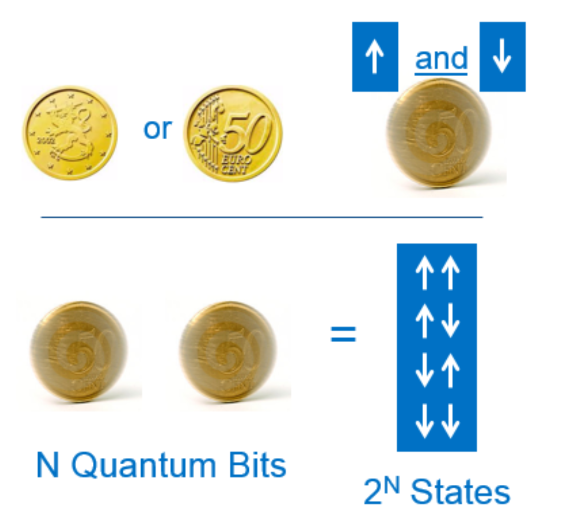
To better understand how a quantum computer works, it helps to compare the basic unit of quantum information, a qubit, with the well-known classical binary bit. A binary bit can be in only one of two possible states: a 0 or a 1. This is similar to how we consider the state of a standard coin lying on a table; it is either heads or tails.
Note
Here we focus on the paradigm of gate-based quantum computing using qubits. Other types of quantum systems are not directly supported by the Intel® Quantum SDK.
In this analogy we consider the state of a quantum coin to be “spinning” on the table top; that is, it is in neither the heads nor the tails state, it is in both states at the same time. In the quantum realm, this concept is called superposition: a qubit is simultaneously in both the 0 and the 1 state (in quantum mechanics, these are referred to as \(\ket{0}, \ket{1}\)). In fact, a qubit is in a linear combination of these two states. So in some sense, a qubit is more like a weighted spinning coin; it has some chance of being in the 0 state, and some chance of being in the 1 state. In quantum mechanics we often write this scenario as:
where \(\ket{\psi}\) represents the state of the qubit and \(\alpha\) and \(\beta\) represent the probability “amplitude” of the qubit being in the \(\ket{0}\) or the \(\ket{1}\) state, respectively. Actually, the \(\alpha\) and \(\beta\) coefficients are complex numbers, and the square of their absolute values (as in, \(\vert\alpha\vert^2\) and \(\vert\beta\vert^2\)) represents the real-world probability of that qubit being in the \(\ket{0}\) or the \(\ket{1}\) states, respectively. Since there are only 2 possible states, we know that \(\vert \alpha \vert ^2 + \vert \beta \vert ^2 = 1\), which simply means there is a 100% chance that the qubit is in either the \(\ket{0}\) or the \(\ket{1}\) state. Just as we can stop a spinning coin at any time with our finger, we can also measure the state of a qubit \(\ket{\psi}\) to see exactly which state it is in at a given time: we represent this measurement with a very simple quantum circuit diagram:
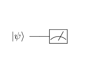
Note
This quantum circuit diagram represents measuring an arbitrary single-qubit state \(\ket{\psi}\). Quantum circuit diagrams are read left-to-right. More operations on a single qubit extend the circuit horizontally, and more qubits are added vertically.
Immediately upon measuring the qubit’s state, we will see that is it in either the \(\ket{0}\) state or the \(\ket{1}\) state. The probability the qubit is \(\ket{0}\) is \(\vert \alpha \vert ^2\), and the probability the qubit is \(\ket{1}\) is \(\vert \beta \vert ^2\). An important property of quantum measurements is that they change the state of the underlying qubits, irreversibly collapsing the qubit’s state from a superposition to a single state.
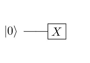
Applying operations like measurements or other quantum gates (such as a qubit “flip”) is fundamental to quantum computing. For example, we can flip the \(\ket{0}\) state to the \(\ket{1}\) state with an X gate, as represented by this circuit diagram:
Furthermore, qubits can be entangled with each other. That is, the combined state of multiple qubits can be correlated. In our coin analogy above, 2 spinning coins could represent 4 possible states via superposition. But if the two spinning coins are entangled, the result of one coin will necessarily inform us of the result of the other. In the similar case of measuring an entangled Bell pair of qubits, measuring the state of one qubit lets us know the state of the second qubit, even without measuring the second qubit.
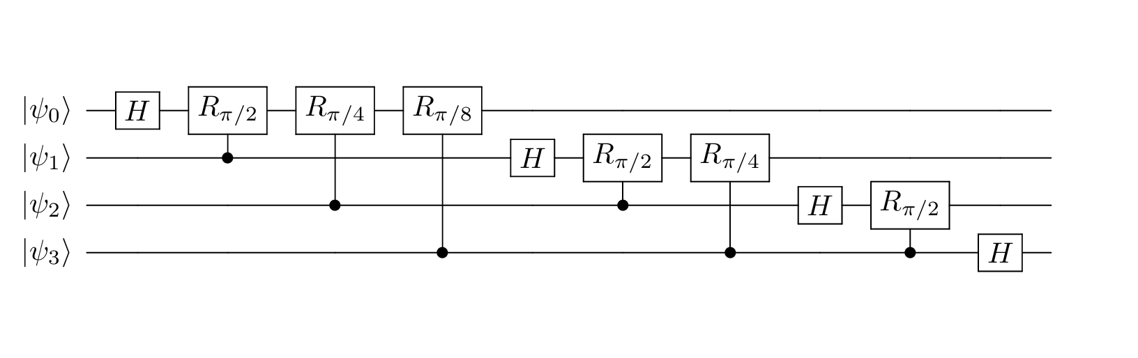
These two properties, superposition and entanglement, enable quantum computers to solve certain problems far more efficiently than a classical computer. Generally speaking, quantum computing is performing quantum operations on qubits to solve these interesting problems. One example is applying a Quantum Fourier Transform (QFT); with only \(O(n^2)\) gates, specifically the Hadamard and phase-shift gates (see the quantum gates and the QFT sample sections for more details), we can apply a Fourier transform on \(O(2^n)\) amplitudes. The corresponding 4-qubit QFT circuit diagram looks like this:
To learn more about quantum computing and how to develop quantum algorithms like the one above, see suggestions in the Getting Started Guide.