Diagnosis
Diagnosis Introduction
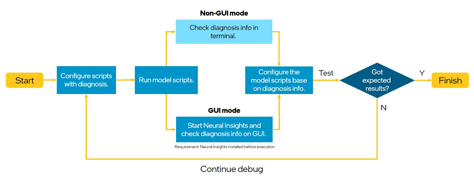
The diagnosis feature provides methods to debug the accuracy loss during quantization and profile the performance gap during benchmark. There are 2 ways to diagnose a model with Intel® Neural Compressor. First is non-GUI mode that is described below and second is GUI mode with Neural Insights component.
The workflow is described in the diagram below. First we have to configure scripts with diagnosis, then run them and check diagnosis info in the terminal. Test if the result is satisfying and repeat the steps if needed.
Supported Feature Matrix
| Types | Diagnosis data | Framework | Backend |
|---|---|---|---|
| Post-Training Static Quantization (PTQ) | weights and activations | TensorFlow | TensorFlow/Intel TensorFlow |
| ONNX Runtime | QLinearops/QDQ | ||
| Benchmark Profiling | OP execute duration | TensorFlow | TensorFlow/Intel TensorFlow |
| ONNX Runtime | QLinearops/QDQ |
Get Started
Install Intel® Neural Compressor
First you need to install Intel® Neural Compressor.
git clone https://github.com/intel/neural-compressor.git
cd neural-compressor
pip install -r requirements.txt
python setup.py install
Modify script
Modify quantization/benchmark script to run diagnosis by adding argument diagnosis set to True to PostTrainingQuantConfig/BenchmarkConfig as shown below.
Quantization diagnosis
config = PostTrainingQuantConfig(diagnosis=True, ...)
Benchmark diagnosis
config = BenchmarkConfig(diagnosis=True, ...)
Example
Below it is explained how to run diagnosis for ONNX ResNet50 model.
Prepare dataset
Download dataset ILSVR2012 validation Imagenet dataset.
Download label:
wget http://dl.caffe.berkeleyvision.org/caffe_ilsvrc12.tar.gz
tar -xvzf caffe_ilsvrc12.tar.gz val.txt
Run quantization script
Then execute script with quantization API in another terminal with –diagnose flag.
python examples/onnxrt/image_recognition/resnet50_torchvision/quantization/ptq_static/main.py \
  --model_path=/path/to/resnet50_v1.onnx/ \
  --dataset_location=/path/to/ImageNet/ \
  --label_path=/path/to/val.txt/
  --tune
  --diagnose
Run benchmark script
To run profiling execute script with parameters shown in the command below.
python examples/onnxrt/image_recognition/resnet50_torchvision/quantization/ptq_static/main.py \
--model_path=/path/to/resnet50_v1.onnx/ \
--dataset_location=/path/to/ImageNet/ \
--label_path=/path/to/val.txt/
--mode=performance \
--benchmark \
--diagnose
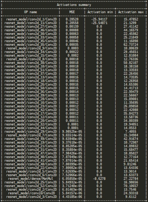
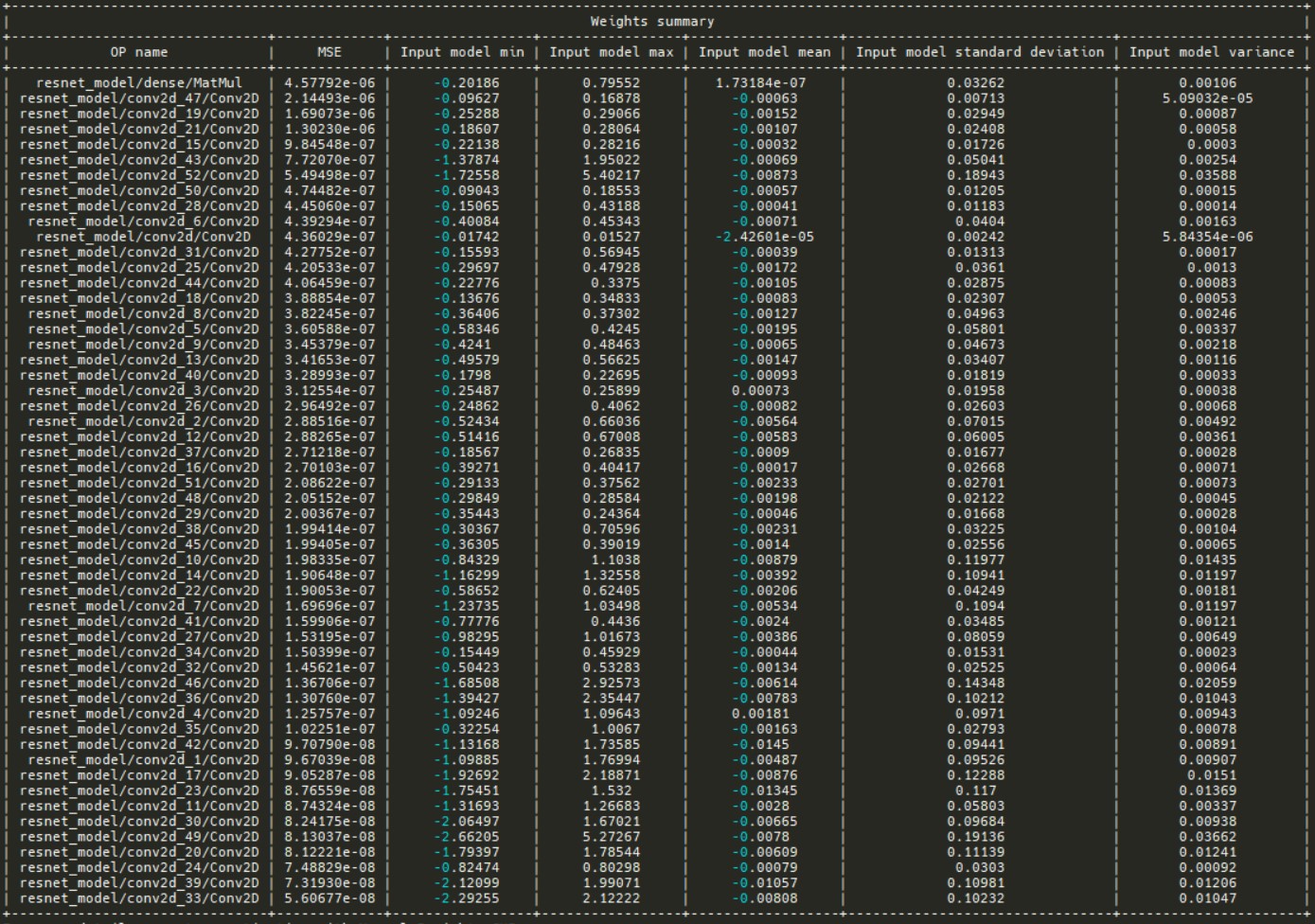
See quantization data
After script’s execution you will see the results in your terminal. In the activations summary you can see a table with OP name, MSE (mean squared error), activation minimum and maximum sorted by MSE.
In the weights summary table there are parameters like minimum, maximum, mean, standard deviation and variance for input model. The table is also sorted by MSE.
How to do diagnosis
Neural Compressor diagnosis mode provides weights and activation data that includes several useful metrics for diagnosing potential losses of model accuracy.
Parameter description
Data is presented in the terminal in form of table where each row describes single OP in the model. We present such quantities measures like:
MSE - Mean Squared Error - it is a metric that measures how big is the difference between input and optimized model’s weights for specific OP.
$$ MSE = \sum_{i=1}^{n}(x_i-y_i)^2 $$
Input model min - minimum value of the input OP tensor data
$$ \min{\vec{x}} $$
Input model max - maximum value of the input OP tensor data
$$ \max{\vec{x}} $$
Input model mean - mean value of the input OP tensor data
$$ \mu =\frac{1}{n} \sum_{i=1}^{n} x_{i} $$
Input model standard deviation - standard deviation of the input OP tensor data
$$ \sigma =\sqrt{\frac{1}{n}\sum\limits_{i=1}^n (x_i - \mu)} $$
Input model variance - variance of the input OP tensor data
$$ Var = \sigma^2 $$
where, $x_i$ - input OP tensor data, $y_i$ - optimized OP tensor data, $\mu_x$ - input model mean, $\sigma_x$ - input model variance
Diagnosis suggestions
Check the nodes with MSE order. High MSE usually means higher possibility of accuracy loss happened during the quantization, so fallback those Ops may get some accuracy back.
Check the Min-Max data range. An dispersed data range usually means higher accuracy loss, so we can also try to full back those Ops.
Check with the other data and find some outliers, and try to fallback some Ops and test for the quantization accuracy.
Note: We can’t always trust the debug rules, it’s only a reference, sometimes the accuracy regression is hard to explain.
Fallback setting example
from neural_compressor import quantization, PostTrainingQuantConfig

op_name_dict = {"v0/cg/conv0/conv2d/Conv2D": {"activation": {"dtype": ["fp32"]}}}
config = PostTrainingQuantConfig(
    diagnosis=True,
    op_name_dict=op_name_dict,
)
q_model = quantization.fit(
    model,
    config,
    calib_dataloader=dataloader,
    eval_func=eval,
)
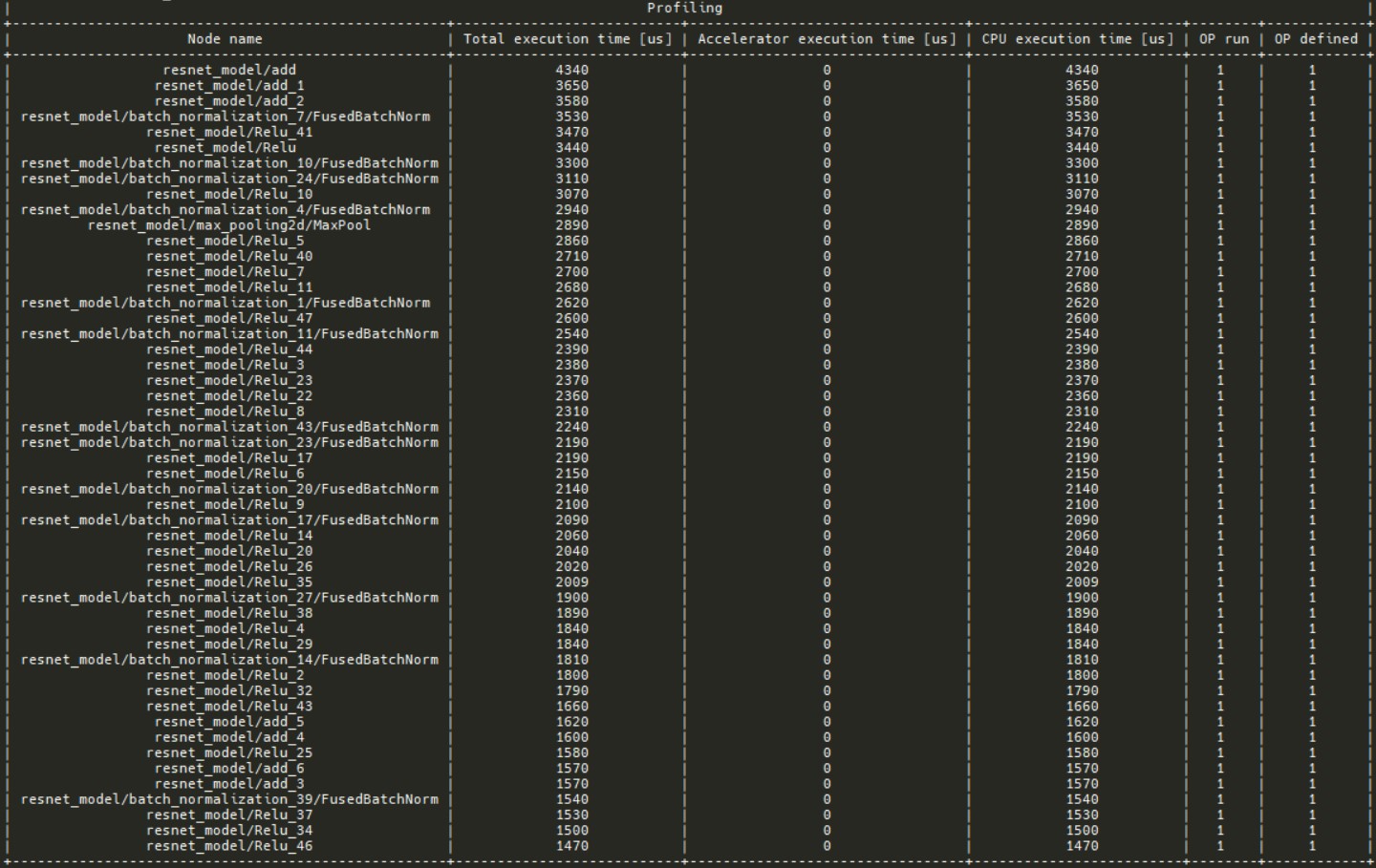
See profiling data
In profiling section there is a table with nodes sorted by total execution time. It is possible to check which operations take the most time.