Quantization

1. Introduction

2. Quantization Fundamentals

3. Quantization methods

   • Dynamic Quantization

   • Static Quantization

   • Smooth Quantization

   • Weight Only Quantization

   • Quantization Aware Training

   • Accuracy Aware Tuning

Introduction

Quantization is a very popular deep learning model optimization technique invented for improving the speed of inference. It minimizes the number of bits required by converting a set of real-valued numbers into the lower bit data representation, such as int8 and int4, mainly on inference phase with minimal to no loss in accuracy. This way reduces the memory requirement, cache miss rate, and computational cost of using neural networks and finally achieve the goal of higher inference performance. On Intel 3rd Gen Intel Xeon Scalable Processors, user could expect up to 4x theoretical performance speedup. We expect further performance improvement with Intel Advanced Matrix Extensions on 4th Gen Intel Xeon Scalable Processors.

Quantization Fundamentals

The equation of quantization is as follows:

$$ X_{int8} = round(X_{fp32}/S) + Z \tag{1} $$

where $X_{fp32}$ is the input matrix, $S$ is the scale factor, $Z$ is the integer zero point.

Symmetric & Asymmetric

---

asymmetric quantization, in which we map the min/max range in the float tensor to the integer range. Here int8 range is [-128, 127], uint8 range is [0, 255].

here:

If INT8 is specified, $Scale = (|X_{f_{max}} - X_{f_{min}}|) / 127$ and $ZeroPoint = -128 - X_{f_{min}} / Scale$.

or

If UINT8 is specified, $Scale = (|X_{f_{max}} - X_{f_{min}}|) / 255$ and $ZeroPoint = - X_{f_{min}} / Scale$.

---

Symmetric quantization, in which we use the maximum absolute value in the float tensor as float range and map to the corresponding integer range.

The math equation is like:

here:

If INT8 is specified, $Scale = max(abs(X_{f_{max}}), abs(X_{f_{min}})) / 127$ and $ZeroPoint = 0$.

or

If UINT8 is specified, $Scale = max(abs(X_{f_{max}}), abs(X_{f_{min}})) / 255$ and $ZeroPoint = 128$.

NOTE

Sometimes the reduce_range feature, that’s using 7 bit width (1 sign bit + 6 data bits) to represent int8 range, may be needed on some early Xeon platforms, it’s because those platforms may have overflow issues due to fp16 intermediate calculation result when executing int8 dot product operation. After AVX512_VNNI instruction is introduced, this issue gets solved by supporting fp32 intermediate data.

---

Quantization Scheme in TensorFlow

• Symmetric Quantization

  • int8: scale = 2 * max(abs(rmin), abs(rmax)) / (max(int8) - min(int8) - 1)

  • uint8: scale = max(rmin, rmax) / (max(uint8) - min(uint8))

---

Quantization Scheme in PyTorch

• Symmetric Quantization

  • int8: scale = max(abs(rmin), abs(rmax)) / (float(max(int8) - min(int8)) / 2)

  • uint8: scale = max(abs(rmin), abs(rmax)) / (float(max(int8) - min(int8)) / 2)

• Asymmetric Quantization

  • uint8: scale = (rmax - rmin) / (max(uint8) - min(uint8)); zero_point = min(uint8) - round(rmin / scale)

---

Quantization Scheme in IPEX

• Symmetric Quantization

  • int8: scale = 2 * max(abs(rmin), abs(rmax)) / (max(int8) - min(int8) - 1)

  • uint8: scale = max(rmin, rmax) / (max(uint8) - min(uint8))

---

Per-tensor & Per-channel

---

There are several choices of sharing quantization parameters among tensor elements, also called quantization granularity. The coarsest level, per-tensor granularity, is that all elements in the tensor share the same quantization parameters. Finer granularity means sharing quantization parameters per row or per column for 2D matrices and per channel for 3D matrices. Similarly, the finest granularity is that each element has an individual set of quantization parameters.

However, due to the model accuracy and computational consumption, per-tensor or per-channel are usually adopted. In the following part, We will show that per-channel could bring lower quantization loss but has some limitations, that is why normally we use per-channel for weight quantization and per-tensor for activation/input quantization

Per-tensor example

---

Suppose the weight tensor is：

import torch

W = torch.Tensor(
    [
        [0.6839, 0.4741, 0.7451],
        [0.9301, 0.1742, 0.6835],
    ]
)

According to the formula (1), we need scale $S$ and zero point $Z$ to calculate the integer matrix.

$$ S = \frac{X_{max} - X{min}}{2^b -1} \tag{2} $$

$$ Z = -round(X_{min/}/S) \tag{3} $$

The per-tensor quantization function is:

def quantize(x, num_bits=8):
    q_min, q_max = 0, 2.0**num_bits - 1.0
    scale = (torch.max(x) - torch.min(x)) / (2**num_bits - 1)
    scale = torch.clip(scale, min=1e-5)
    zp = torch.round(0 - (torch.min(x)) / scale)
    q_x = x / scale + zp
    q_x.clamp_(q_min, q_max).round_()
    print(f"scale = {scale}, zp = {zp}")
    return q_x, scale, zp

Then we can get the quantized $W_{q}$

>>> W_q, scale, zp = quantize(W)
scale = 0.00296431384049356, zp = -59.0
>>> W_q
tensor([[172., 101., 192.],
        [255.,   0., 172.]])

With the value of scale and zp, we can dequantize the tensor.

def dequantize(q_x, scale, zp):
    return scale * (q_x - zp)

>>> W_dq = dequantize(W_q, 0.001, -50)
>>> W_dq
tensor([[0.2220, 0.1510, 0.2420],
        [0.2570, 0.0500, 0.1890]])
>>> loss = torch.nn.MSELoss()(W_dq, W)
>>> loss.item()
0.1983354538679123

>>> W_dq = dequantize(W_q, scale, zp)
>>> W_dq
tensor([[0.6848, 0.4743, 0.7440],
        [0.9308, 0.1749, 0.6848]])
>>> loss = torch.nn.MSELoss()(W_dq, W)
>>> loss.item()
7.385297635664756e-07

The difference between $W$ and $W_{dq}$ shows that quantization affects precision and appropriate values of scale and zero point will reduce the loss of precision.

Per-channel example

---

Similarly, the example of per-channel quantization is as follows:

def quantize_per_channel(x, num_bits=8):
    q_min, q_max = 0, 2.0**num_bits - 1.0
    x_tmp = x.detach().reshape(x.shape[0], -1)
    scales = x_tmp.max(dim=-1, keepdim=True)[0] / (2**num_bits - 1)
    zp = torch.round(0 - x_tmp.min(dim=-1, keepdim=True)[0].divide(scales))
    q_x = x_tmp.divide(scales) + zp
    q_x.clamp_(q_min, q_max).round_()
    print(f"scales = {scales}, \n zp = {zp}")
    return q_x, scales, zp


def dequantize_per_channel(q_x, scales, zp):
    print(q_x, scales, zp)
    print(scales * (q_x - zp))
    return scales * (q_x - zp)

>>>W_q, scales, zp = quantize_per_channel(W)
scale = tensor([[0.0029],
        [0.0036]]), 
zp = tensor([[-162.],
        [ -48.]])
>>>W_q
tensor([[ 72.,   0.,  93.],
        [207.,   0., 139.]])

>>>W_dq = dequantize_per_channel(W_q, scales, zp)
>>>W_dq
tensor([[0.6837, 0.4734, 0.7451],
        [0.9301, 0.1751, 0.6821]])

And the loss is

>>> loss = torch.nn.MSELoss()(W_dq, W)
>>> loss.item()
5.637690492221736e-07

Through this example, we can see that per-channel quantization has finer granularity and has lower loss (loss 5.6376e-07 for per-channel quantization and 7.3852e-07 for per-tensor quantization).

Matmul quantization example

---

For a linear layer in most model, $Y=X \cdot W$, we can quantize both the weights and activations in order to reduce the storage and accelerate inference. Using per-tensor scale quantization to show the process.

def quantize_per_tensor_absmax(x, n_bits=8):
    scales = x.abs().max()
    q_max = 2 ** (n_bits - 1) - 1
    scales.clamp_(min=1e-5).div_(q_max)
    q_x = x / scales
    q_x = q_x.clamp_(-q_max, q_max).round_()
    return q_x, scales


def dequantize(q_x, scale):
    return scale * q_x

Randomly initialize the $W$ and $Y$, then calculate the result of $Y=X \cdot W$

>>>W = torch.rand(2, 3, dtype=torch.float32)
>>>X = torch.rand(3, 4, dtype=torch.float32)
>>>W
tensor([[0.0806, 0.7589, 0.6038],
        [0.3815, 0.5040, 0.7174]])
>>>X
tensor([[0.5444, 0.5826, 0.7772, 0.5555],
        [0.3740, 0.3253, 0.0698, 0.1381],
        [0.5972, 0.0086, 0.0737, 0.8298]])
>>>Y = torch.matmul(W, X)
>>>Y
tensor([[0.6883, 0.2991, 0.1601, 0.6506],
        [0.8246, 0.3924, 0.3845, 0.8768]])

Quantize weight and activation, matmul(quantize(X), quantize(Y))

>>>W_q, W_scale = quantize_per_tensor_absmax(W)
>>>X_q, X_scale = quantize_per_tensor_absmax(X)
>>>print(f'{W_q}\n{W_scale.item()}')
>>>print(f'{X_q}\n{X_scale.item()}')
tensor([[ 13., 127., 101.],
        [ 64.,  84., 120.]])
0.0059755356051027775
tensor([[ 83.,  89., 119.,  85.],
        [ 57.,  50.,  11.,  21.],
        [ 91.,   1.,  11., 127.]])
0.006533813662827015

>>>Y_q = torch.matmul(W_q, X_q)
>>>Y_q
tensor([[17509.,  7608.,  4055., 16599.],
        [21020., 10016.,  9860., 22444.]])
>>>Y_dq = dequantize(Y_q, W_scale * X_scale)
>>>Y_dq
tensor([[0.6836, 0.2970, 0.1583, 0.6481],
        [0.8207, 0.3911, 0.3850, 0.8763]])

Dynamic Quantization

The weights of the neural network get quantized into int8 format from float32 format offline. The activations of the neural network is quantized as well with the min/max range collected during inference runtime.

This approach is widely used in dynamic length neural networks, like NLP model.

Static Quantization

Compared with post training dynamic quantization, the min/max range in weights and activations are collected offline on a so-called calibration dataset. This dataset should be able to represent the data distribution of those unseen inference dataset. The calibration process runs on the original fp32 model and dumps out all the tensor distributions for Scale and ZeroPoint calculations. Usually preparing 100 samples are enough for calibration.

This approach is major quantization approach people should try because it could provide the better performance comparing with post training dynamic quantization.

Smooth Quantization

Per-channel limitation

---

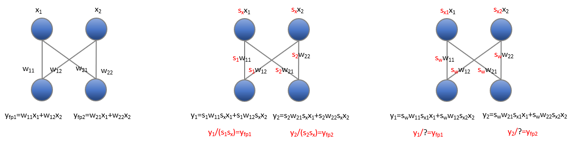
Though per-channel quantization could bring lower quantization error, we could not apply it for activations due to the difficulty of the dequantization. We would prove it in the following image and the zero point of quantization would be ignored for simplicity.

The image on the left presents a normal linear forward with 1x2 input $x$ and 2x2 weight $w$. The results $y$ could be easily obtained by simple mathematics. In the middle image, we apply per-tensor quantization for activations and per-channel quantization for weights; the results after quantization that are denoted by $y_1$ and $y_2$, could be easily dequantized to the float results $y_{fp1}$ and $y_{fp2}$ by per channel scale $1.0/s_1s_x$ and $1.0/s_2s_x$. However, after applying per-channel quantization for activation (right image), we could not dequantize the $y_1$ and $y_2$ to float results.

---

In the previous subsection, we have explained why per-channel quantization could not be applied for activation, even though it could lead to lower quantization loss. However, the quantization error loss of activation plays an important role in the accuracy loss of model quantization[1][6][7].

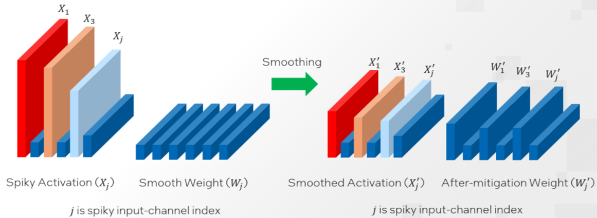
To reduce the quantization loss of activations, lots of methods have been proposed. In the following, we briefly introduce SPIQ[6], Outlier Suppression[7] and Smoothquant[1]. All these three methods share a similar idea to migrate the difficulty from activation quantization to weight quantization but differ in how much difficulty to be transferred.

So the first question is how to migrate the difficulty from activation to weights? The solution is straightforward, that is to convert the network to an output equivalent network that is presented in the image below and apply quantization to this equivalent network. The intuition is that each channel of activation could be scaled to make it more quantization-friendly, similar to a fake per-channel activation quantization.

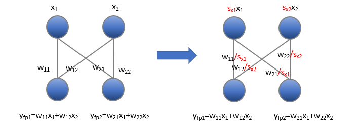
Please note that this conversion will make the quantization of weights more difficult, because the scales attached to weights shown above are per-input-channel, while quantization of weights is per-output-channel or per-tensor.

So the second question is how much difficulty to be migrated, that is how to choose the conversion per-channel scale $s_{x1}$ and $s_{x2}$ from the above image. Different works adopt different ways.

SPIQ just adopts the quantization scale of activations as the conversion per-channel scale.

Outlier suppression adopts the scale of the preceding layernorm as the conversion per-channel scale.

Smoothquant introduces a hyperparameter $\alpha$ as a smooth factor to calculate the conversion per-channel scale and balance the quantization difficulty of activation and weight.

$$ s_j = max(|X_j|)^\alpha/max(|W_j|)^{1-\alpha} \tag{4} $$

j is the index of the input channels.

For most of the models such as OPT and BLOOM, $\alpha = 0.5$ is a well-balanced value to split the difficulty of weight and activation quantization. A larger $\alpha$ value could be used on models with more significant activation outliers to migrate more quantization difficulty to weights.

Weight Only Quantization

As large language models (LLMs) become more prevalent, there is a growing need for new and improved quantization methods that can meet the computational demands of these modern architectures while maintaining the accuracy. Compared to normal quantization like W8A8, weight only quantization is probably a better trade-off to balance the performance and the accuracy, since we will see below that the bottleneck of deploying LLMs is the memory bandwidth and normally weight only quantization could lead to better accuracy.

Model inference: Roughly speaking , two key steps are required to get the model’s result. The first one is moving the model from the memory to the cache piece by piece, in which, memory bandwidth $B$ and parameter count $P$ are the key factors, theoretically the time cost is $P*4 /B$. The second one is computation, in which, the device’s computation capacity $C$ measured in FLOPS and the forward FLOPs $F$ play the key roles, theoretically the cost is $F/C$.

Text generation: The most famous application of LLMs is text generation, which predicts the next token/word based on the inputs/context. To generate a sequence of texts, we need to predict them one by one. In this scenario, $F\approx P$ if some operations like bmm are ignored and past key values have been saved. However, the $C/B$ of the modern device could be to 100X, that makes the memory bandwidth as the bottleneck in this scenario.

Besides, as mentioned in many papers[1][2], activation quantization is the main reason to cause the accuracy drop. So for text generation task, weight only quantization is a preferred option in most cases.

Theoretically, round-to-nearest (RTN) is the most straightforward way to quantize weight using scale maps. However, when the number of bits is small (e.g. 3), the MSE loss is larger than expected. A group size is introduced to reduce elements using the same scale to improve accuracy.

There are many excellent works for weight only quantization to improve its accuracy performance, such as AWQ[3], GPTQ[4], AutoRound[8]. Neural compressor integrates these popular algorithms in time to help customers leverage them and deploy them to their own tasks.

Quantization Aware Training

Quantization aware training emulates inference-time quantization in the forward pass of the training process by inserting fake quant ops before those quantizable ops. With quantization aware training, all weights and activations are fake quantized during both the forward and backward passes of training: that is, float values are rounded to mimic int8 values, but all computations are still done with floating point numbers. Thus, all the weight adjustments during training are made while aware of the fact that the model will ultimately be quantized; after quantizing, therefore, this method will usually yield higher accuracy than either dynamic quantization or post-training static quantization.

Accuracy Aware Tuning

Accuracy aware tuning is one of unique features provided by Intel(R) Neural Compressor, compared with other 3rd party model compression tools. This feature can be used to solve accuracy loss pain points brought by applying low precision quantization and other lossy optimization methods.

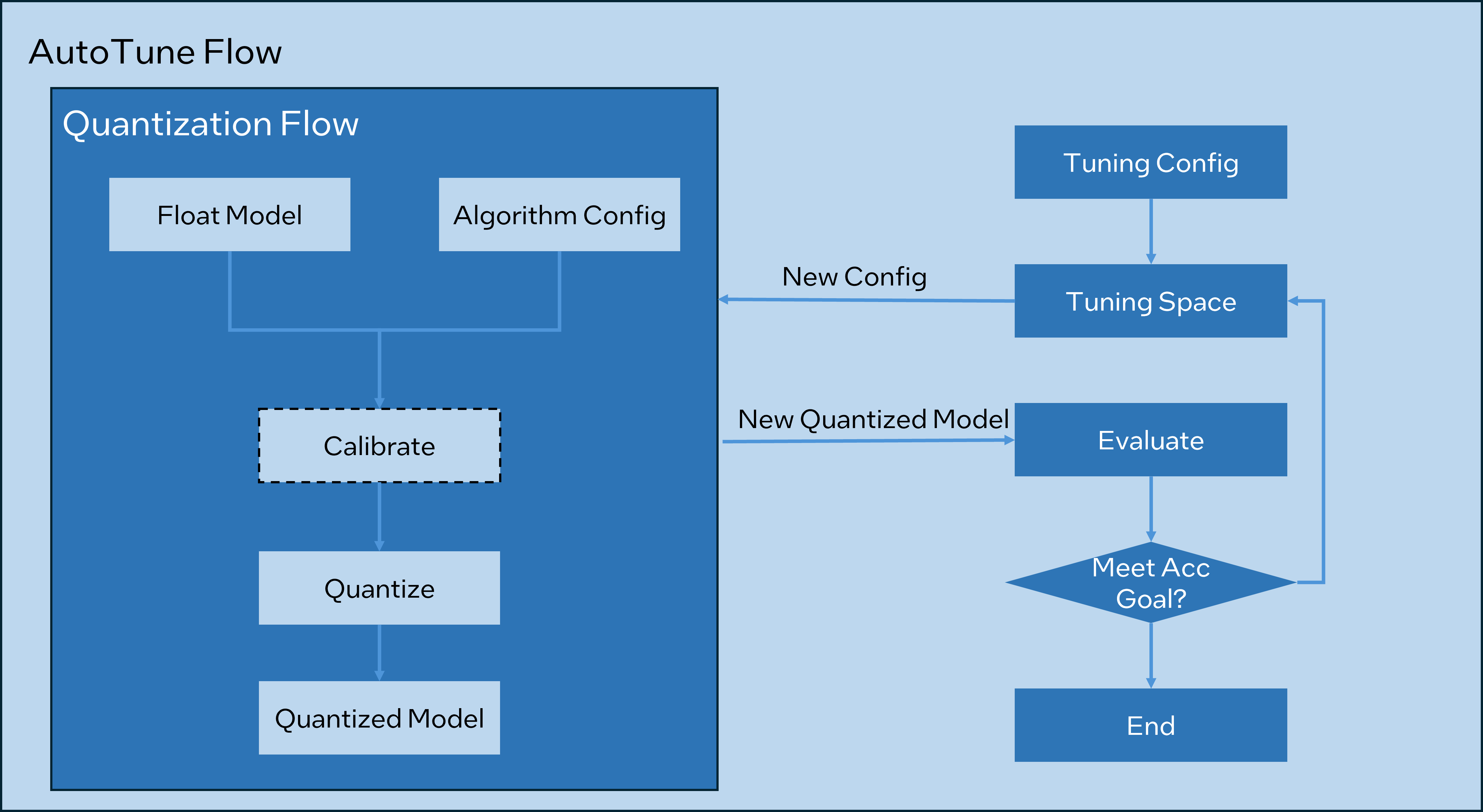
This tuning algorithm creates a tuning space by querying framework quantization capability and model structure, selects the ops to be quantized by the tuning strategy, generates quantized graph, and evaluates the accuracy of this quantized graph. The optimal model will be yielded if the pre-defined accuracy goal is met. The autotune serves as a main interface of this algorithm.

Neural compressor also support to quantize all quantizable ops without accuracy tuning, using quantize_model interface to achieve that.

For supported quantization methods for accuracy aware tuning and the detailed API usage, please refer to the document of PyTorch or TensorFlow respectively.

User could refer to below chart to understand the whole tuning flow.

Reference

[1]. Xiao, Guangxuan, et al. “Smoothquant: Accurate and efficient post-training quantization for large language models.” arXiv preprint arXiv:2211.10438 (2022).

[2]. Wei, Xiuying, et al. “Outlier suppression: Pushing the limit of low-bit transformer language models.” arXiv preprint arXiv:2209.13325 (2022).

[3]. Lin, Ji, et al. “AWQ: Activation-aware Weight Quantization for LLM Compression and Acceleration.” arXiv preprint arXiv:2306.00978 (2023).

[4]. Frantar, Elias, et al. “Gptq: Accurate post-training quantization for generative pre-trained transformers.” arXiv preprint arXiv:2210.17323 (2022).

[5]. Dettmers, Tim, et al. “Qlora: Efficient finetuning of quantized llms.” arXiv preprint arXiv:2305.14314 (2023).

[6]. Yvinec, Edouard, et al. “SPIQ: Data-Free Per-Channel Static Input Quantization.” Proceedings of the IEEE/CVF Winter Conference on Applications of Computer Vision. 2023.

[7]. Wei, Xiuying, et al. “Outlier suppression: Pushing the limit of low-bit transformer language models.” arXiv preprint arXiv:2209.13325 (2022).

[8]. Cheng, Wenhua, et al. “Optimize weight rounding via signed gradient descent for the quantization of llms.” arXiv preprint arXiv:2309.05516 (2023).