Split SGD

Both optimizations for inference workloads and training workloads are within Intel’s optimization scope. Optimizations for train optimizer functions are an important perspective. The optimizations use a mechanism called Split SGD and take advantage of BFloat16 data type and operator fusion. Optimizer adagrad, lamb and sgd are supported.

BFloat16

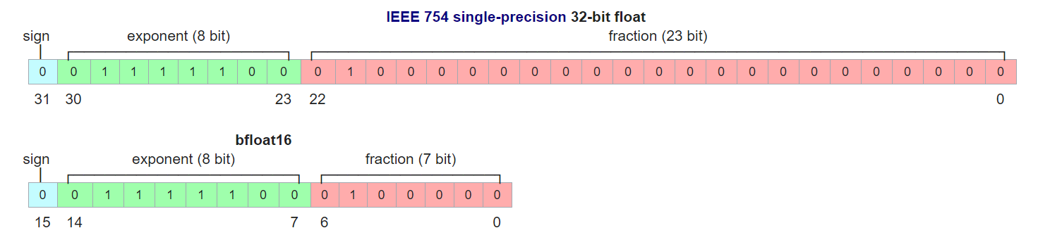
The figure below shows definition of Float32 (top) and BFloat16 (bottom) data types. Compared to Float32, BFloat16 is only half as long, and thus saves half the memory. It is supported natively at the instruction set level to boost deep learning workloads from the 3rd Generation of Intel® Xeon® Scalable Processors. It is compatible to Float32 since both have the same bit length for “sign” and “exponent” part. BFloat16 only has a 7-bit “mantissa” part while Float32 has 23 bits. BFloat16 has the same capacity to represent “digit ranges” with that of Float32, but has a shorter “precision” part.

An advantage of BFloat16 is that it saves memory and reduces computation workload, but the fewer mantissa bits brings negative effects as well. Let’s use an “ADD” operation as an example to explain the disadvantage. To perform addition of 2 floating point numbers, we need to shift the mantissa part of the numbers left or right to align their exponent parts. Since BFloat16 has a shorter mantissa part, it is much easier than Float32 to lose its mantissa part after the shifting, and thus cause an accuracy loss issue.

Let’s use the following two decimal numbers x and y as an example. We first do the calculation in a high precision data type (10 valid numbers after decimal point).

$$\begin{array}{rl}x& =0.1234500000\ast {10}^{10}\\ y& =0.1234500000\ast {10}^5\\ x+y& =0.1234500000\ast {10}^{10}+0.1234500000\ast {10}^5\\ & =0.1234500000\ast {10}^{10}+0.0000012345\ast {10}^{10}\\ & =0.1234512345\ast {10}^{10}\end{array}$$

This makes sense because after shifting y right by 5 digits, the fraction part is still there.

Let’s do the calculation using a low precision data type (5 valid numbers after decimal point):

$$\begin{array}{rl}x& =0.12345\ast {10}^{10}\\ y& =0.12345\ast {10}^5\\ x+y& =0.12345\ast {10}^{10}+0.12345\ast {10}^5\\ & =0.12345\ast {10}^{10}+0.00000\ast {10}^{10}\\ & =0.12345\ast {10}^{10}\end{array}$$

Since the data type has only 5 digits for the fraction part, after shifting y by 5 digits, its fraction part is fully removed. This causes significant accuracy loss and, buy their nature, is a drawback of lower-precision data types.

Stochastic Gradient Descent (SGD)

Basically, training involves 3 steps:

1. Forward propagation: Performance inference once and compare the results with ground truth to get loss number.

2. Backward propagation: Utilize chain rule to calculate gradients of parameters based on the loss number.

3. Parameter update: Update value of parameters by gradients along with calculated loss values.

The training is actually a loop of these 3 steps in sequence until the loss number meets requirements or after a determined timeout duration. The Stochastic Gradient Descent (SGD) is most widely used at the 3rd step to update parameter values. To make it easy to understand, the 3rd step is described as the following formula:

$$W=W+\alpha \ast gW$$

Where $W$ denotes parameters to be updated. $gW$ denotes gradient received during backward propagation and $\alpha$ denotes learning rate.

Split SGD

Since the addition applied in SGD is repeated, because of the low precision data loss mentioned earlier, if both the $W$ and $gW$ are stored in BFloat16 data type, we will most likely lose valid bits and make the training results inaccurate. Using FP32 master parameters is a common practice for avoiding the round-off errors at parameter update step. To keep FP32 master parameters, we have 3 design choices: 1. Only save FP32 parameters: For this choice, we need introduce additional FP32->BF16 cast at each iter to get benefit from BF16 at forward and backward propagation steps. 2. Save both FP32 and BF16 parameters: BF16 parameter is used at forward and backward propagation steps. Use FP32 master parameter at update steps. For this choice we introduce more memory footprint. 3. “Split” choice: In order to get performance benefits with BFloat16 at forward and backward propagation steps, while avoiding increase the memory footprint, we propose the mechanism “Split SGD”.

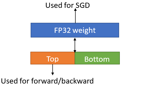
The idea is to “split” a 32-bit floating point number into 2 parts:

1. Top half: First 16 bits can be viewed as exactly a BFloat16 number.

2. Bottom half: Last 16 bits are still kept to avoid accuracy loss.

FP32 parameters are split into “Top half” and “Bottom half”. When performing forward and backward propagations, the Top halves are used to take advantage of Intel BFloat16 support. When performing parameter update with SGD, we concatenate the Top half and the Bottom half to recover the parameters back to FP32 and then perform regular SGD operations.

It is a common practice to use FP32 for master parameters in order to avoid round-off errors with BF16 parameter update. SplitSGD is an optimization of storing FP32 master parameters with reduced memory footprint.

The following pseudo code illustrates the process of Split SGD.

fp32_w = concat_fp32_from_bf16(bf16_w, trail)
fp32_gw = bf16_gw.float()
fp32_w += α* fp32_gw (sgd step without weight_dacay, momentum)
bf16_w, trail = split_bf16_from_fp32(fp32_w)