Graph Optimization

Most Deep Learning models could be described as a directed acyclic graph (DAG). How to optimize a deep learning model from graph perspective is a natural consideration. Comparing to operator optimization and algorithm optimization, graph optimization is at a higher level. It not only convers the graph model itself but also involves runtime operations. From operator perspective, the graph optimization involves operator fusing and constant folding. From runtime perspective, the graph optimization involves operator scheduling, computation resources management, and memory mangement.

Currently, the Intel Extension for PyTorch focuses on operator-related graph optimizations. Regarding to the runtime related optimizations, the extension provides some experimental features. Please refer to the runtime extension for more details about runtime optimization.

Fusion

FP32 and BF16 fusion patterns

Conv2D + ReLU
Conv2D + SUM
Conv2D + SUM + ReLU
Conv2D + Sigmoid
Conv2D + Sigmoid + MUL
Conv2D + HardTanh
Conv2D + SiLU
Conv2D + ELU
Conv3D + ReLU
Conv3D + SUM
Conv3D + SUM + ReLU
Conv3D + SiLU
Linear + ReLU
Linear + GELU
Add + LayerNorm
Div + Add + Softmax
Linear + Linear + Linear
View + Transpose + Contiguous + View

INT8 fusion patterns

The ipex.quantization.convert(model, conf, inputs) API will convert an FP32 torch.nn.Module to a quantized JIT ScriptModule according to the given quantization recipes.

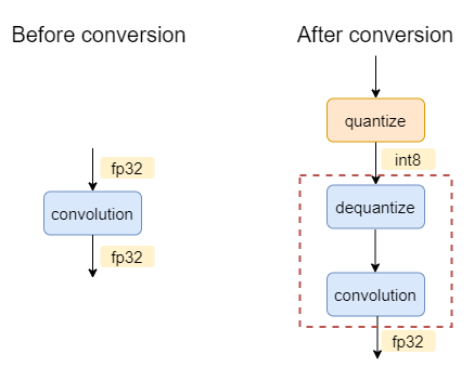
For example, for a FP32 model of one single convolution, the graph before and after conversion will be:

The oneDNN graph backend will select dequantize and convolution into one partition. During execution, this partition will execute a convolution with int8 as input and fp32 as output.

Here listed all the currently supported int8 patterns in Intel® Extension for PyTorch* using oneDNN graph backend:

Patterns with int8 as input and fp32 as output:

dequant -> conv
dequant -> linear
dequant -> conv -> relu
dequant -> conv -> sum
dequant -> conv -> sum -> relu
dequant -> linear -> relu
dequant -> linear -> gelu
dequant -> linear -> sigmoid
dequant -> linear -> sum
dequant -> bmm
dequant -> bmm -> div

Patterns with int8 as input and int8 as output:

dequant -> conv -> quant
dequant -> linear -> quant
dequant -> conv -> relu -> quant
dequant -> conv -> sum -> dequant
dequant -> conv -> sum -> relu -> quant
dequant -> linear -> relu -> quant
dequant -> linear -> gelu -> quant
dequant -> linear -> sigmoid -> quant
dequant -> linear -> sum -> quant
dequant -> bmm -> quant
dequant -> bmm -> div -> quant
dequant -> max_pool2d -> quant

Folding

Stock PyTorch has provided the constant propagation and BatchNormalization folding. And these optimizations will be automatically applied to the jit model by invoking torch.jit.freeze. Take the Resnet50 as the example:

import torch
import torchvision.models as models
model = models.__dict__["resnet50 "](pretrained=True)
model.eval()
x = torch.randn(args.batch_size, 3, 224, 224)
with torch.no_grad():
    model = torch.jit.trace(model, x, check_trace=False).eval()
    # Fold the BatchNormalization and propagate constant
    torch.jit.freeze(model)
    # Print the graph
    print(model.graph_for(x))

If the model owner does not invoke the torch.jit.freeze, the BatchNormalization still exists on the graph. Otheriwse, the BatchNormalization will be folded on the graph to save the compuation and then improve the performance. Please refer to the Constant Folding Wikipedia page for more details.

Ease-of-use graph optimization API

The graph optimizations of Intel® Extension for PyTorch* are enabled by default. Users could disable it by calling:

ipex.enable_onednn_fusion(False)

FP32 and BF16 models

import torch
import torchvision.models as models

# Import the Intel Extension for PyTorch
import intel_extension_for_pytorch as ipex

model = models.__dict__["resnet50 "](pretrained=True)
model.eval()

# Apply some fusions at the front end
model = ipex.optimize(model, dtype=torch.float32)

x = torch.randn(args.batch_size, 3, 224, 224)
with torch.no_grad():
    model = torch.jit.trace(model, x, check_trace=False).eval()
    # Fold the BatchNormalization and propagate constant
    torch.jit.freeze(model)
    # Print the graph
    print(model.graph_for(x))

Compared the original code, the model launcher just needs to add few lines of code, the extension will automatically acceletate the model. Regarding the RN50, the extension will automatically fuse the Conv + ReLU and Conv + Sum + ReLU as ConvReLU and ConvSumReLU. If you check the output of graph_for, you will observe the fused operators.

INT8 models

import torch
import intel_extension_for_pytorch as ipex


# First-time quantization flow 
# define the model 
def MyModel(torch.nn.Module): 
  … 

# construct the model 
model = MyModel(…) 
conf = ipex.QuantConf(dtype=torch.int8) 
model, conf = ipex.quantization.prepare(model, conf) 
for images in calibration_data_loader(): 
  with ipex.quantization.calibrate(conf): # here, conf is in/out, populated with observed statistics 
    model(images) 
conf.save(‘int8_conf.json’, default_recipe=True) # optional: save the configuration for later use 
model = ipex.quantization.convert(model, conf, sample_image) 

# run the model 
output = model(images) 

# Deployment 
import intel_extension_for_pytorch as ipex
conf = ipex.QuantConf(‘int8_conf.json’) 
model = ipex.quantization.convert(model, conf, sample_image) 
output = model(images) 